EDA on Numerical Data#
%config InlineBackend.figure_format='retina'
import logging
from ekorpkit import eKonf

logging.basicConfig(level=logging.WARNING)
print("version:", eKonf.__version__)
print("is notebook?", eKonf.is_notebook())
print("is colab?", eKonf.is_colab())
print("evironment varialbles:")
eKonf.print(eKonf.env().dict())
version: 0.1.33+20.g8433774.dirty
is notebook? True
is colab? False
evironment varialbles:
{'EKORPKIT_CONFIG_DIR': '/workspace/projects/ekorpkit-book/config',
 'EKORPKIT_DATA_DIR': None,
 'EKORPKIT_PROJECT': 'ekorpkit-book',
 'EKORPKIT_WORKSPACE_ROOT': '/workspace',
 'NUM_WORKERS': 230}
data_dir = "../data/fomc"
Load preprocessed data#
econ_data = eKonf.load_data("econ_data2.parquet", data_dir)
econ_data.tail()
| unscheduled | forecast | confcall | speaker | rate | rate_change | rate_decision | rate_changed | GDP | GDP_diff_prev | ... | Rate | Taylor | Balanced | Inertia | Taylor-Rate | Balanced-Rate | Inertia-Rate | Taylor_diff | Balanced_diff | Inertia_diff | |
|---|---|---|---|---|---|---|---|---|---|---|---|---|---|---|---|---|---|---|---|---|---|
| date | |||||||||||||||||||||
| 2021-11-03 | False | False | False | Jerome Powell | 0.25 | 0.00 | 0.0 | 0 | 19478.893 | 0.570948 | ... | 0.25 | 5.747177 | 4.940210 | -0.528532 | 5.497177 | 4.690210 | -0.778532 | 0.0 | 0.0 | 0.0 |
| 2021-12-15 | False | True | False | Jerome Powell | 0.25 | 0.00 | 0.0 | 0 | 19478.893 | 0.570948 | ... | 0.25 | 6.472329 | 5.665362 | -0.637304 | 6.222329 | 5.415362 | -0.887304 | 0.0 | 0.0 | 0.0 |
| 2022-01-26 | False | False | False | Jerome Powell | 0.25 | 0.00 | 0.0 | 0 | 19478.893 | 0.570948 | ... | 0.25 | 7.222928 | 6.415961 | -0.749894 | 6.972928 | 6.165961 | -0.999894 | 0.0 | 0.0 | 0.0 |
| 2022-03-16 | False | True | False | Jerome Powell | 0.50 | 0.25 | 1.0 | 1 | 19806.290 | 1.680778 | ... | 0.25 | 8.499377 | 8.267766 | -1.027665 | 8.249377 | 8.017766 | -1.277665 | 0.0 | 0.0 | 0.0 |
| 2022-05-04 | False | False | False | Jerome Powell | 1.00 | 0.50 | 1.0 | 1 | 19735.895 | -0.355417 | ... | 0.50 | 8.094924 | 7.420939 | -0.688141 | 7.594924 | 6.920939 | -1.188141 | 0.0 | 0.0 | 0.0 |
5 rows × 58 columns
EDA on numerical data#
# Add previous rate decision to see inertia effect
econ_data["Rate Decision"] = econ_data["rate_decision"].map(
    lambda x: "Cut" if x <= -1 else "Hike" if x >= 1 else "Hold"
)
econ_data["rate_decision"] = econ_data["rate_decision"].map(
    lambda x: -1 if x <= -1 else 1 if x >= 1 else 0
)
econ_data["prev_decision"] = econ_data["rate_decision"].shift(1)
econ_data["next_decision"] = econ_data["rate_decision"].shift(-1)
econ_data[["Rate Decision", "rate_decision", "prev_decision", "next_decision"]].head()
| Rate Decision | rate_decision | prev_decision | next_decision | |
|---|---|---|---|---|
| date | ||||
| 1982-10-05 | Cut | -1 | NaN | -1.0 |
| 1982-11-16 | Cut | -1 | -1.0 | 0.0 |
| 1982-12-21 | Hold | 0 | -1.0 | 0.0 |
| 1983-01-14 | Hold | 0 | 0.0 | 0.0 |
| 1983-01-21 | Hold | 0 | 0.0 | 0.0 |
econ_data.describe()
| rate | rate_change | rate_decision | rate_changed | GDP | GDP_diff_prev | GDP_diff_year | GDPPOT | GDPPOT_diff_prev | GDPPOT_diff_year | ... | Balanced | Inertia | Taylor-Rate | Balanced-Rate | Inertia-Rate | Taylor_diff | Balanced_diff | Inertia_diff | prev_decision | next_decision | |
|---|---|---|---|---|---|---|---|---|---|---|---|---|---|---|---|---|---|---|---|---|---|
| count | 415.000000 | 415.000000 | 415.000000 | 415.000000 | 415.000000 | 415.000000 | 415.000000 | 415.000000 | 415.000000 | 415.000000 | ... | 415.000000 | 415.000000 | 415.000000 | 415.000000 | 415.000000 | 415.000000 | 415.000000 | 415.000000 | 414.000000 | 414.000000 |
| mean | 3.968976 | -0.019880 | -0.012048 | 0.334940 | 12815.408884 | 0.657814 | 2.523898 | 13018.548855 | 0.643467 | 2.616803 | ... | 3.324700 | 2.893358 | 0.005563 | -0.665962 | -1.097304 | 0.002576 | 0.005238 | -0.002322 | -0.014493 | -0.009662 |
| std | 3.036522 | 0.228714 | 0.579313 | 0.472539 | 3719.399375 | 1.085580 | 2.203739 | 3776.658124 | 0.185616 | 0.756947 | ... | 2.069550 | 2.373858 | 1.899151 | 2.141286 | 0.711029 | 0.058706 | 0.088255 | 0.026755 | 0.577867 | 0.577968 |
| min | 0.000000 | -1.000000 | -1.000000 | 0.000000 | 6804.139000 | -8.937251 | -9.083737 | 7271.207419 | 0.318708 | 1.303969 | ... | 0.000000 | -1.027665 | -4.920215 | -8.061836 | -2.699376 | -0.400621 | -0.400621 | -0.425000 | -1.000000 | -1.000000 |
| 25% | 1.000000 | 0.000000 | 0.000000 | 0.000000 | 9394.834000 | 0.426261 | 1.701703 | 9597.373675 | 0.475884 | 1.915027 | ... | 1.731034 | 0.561801 | -1.470860 | -1.661544 | -1.567363 | 0.000000 | 0.000000 | 0.000000 | 0.000000 | 0.000000 |
| 50% | 4.000000 | 0.000000 | 0.000000 | 0.000000 | 13183.890000 | 0.678051 | 2.673107 | 13014.429940 | 0.642412 | 2.615226 | ... | 3.386536 | 2.788555 | 0.052807 | -0.293935 | -1.130361 | 0.000000 | 0.000000 | 0.000000 | 0.000000 | 0.000000 |
| 75% | 6.000000 | 0.000000 | 0.000000 | 1.000000 | 15781.342000 | 0.988107 | 3.908365 | 16227.234340 | 0.777802 | 3.150223 | ... | 4.723309 | 4.507101 | 1.361705 | 0.475418 | -0.455663 | 0.000000 | 0.000000 | 0.000000 | 0.000000 | 0.000000 |
| max | 11.500000 | 1.125000 | 1.000000 | 1.000000 | 19806.290000 | 7.547535 | 12.226677 | 20003.730000 | 1.058177 | 4.280368 | ... | 8.267766 | 8.901506 | 8.249377 | 8.017766 | -0.037500 | 0.616857 | 1.233715 | 0.060093 | 1.000000 | 1.000000 |
8 rows × 46 columns
econ_data.isnull().sum()
unscheduled      0
forecast         0
confcall         0
speaker          0
rate             0
                ..
Balanced_diff    0
Inertia_diff     0
Rate Decision    0
prev_decision    1
next_decision    1
Length: 61, dtype: int64
Plot rate decision count#
cfg = eKonf.compose("visualize/plot=countplot")
cfg.countplot.x = "Rate Decision"
cfg.figure.figsize = (10, 5)
cfg.ax.title = "Rate Decision Count"
eKonf.instantiate(cfg, data=econ_data)
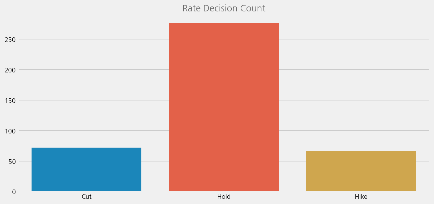
Highly imbalanced to 0 (hold), so need to consider this point. Always predicting 0 (hold) will result in the accuracy of more than 60%.
Correlation#
corr_columns = [
    "rate_decision",
    "next_decision",
    "prev_decision",
    "unscheduled",
    "forecast",
    "confcall",
    "GDP_diff_prev",
    "GDP_diff_year",
    "GDPPOT_diff_prev",
    "GDPPOT_diff_year",
    "PCE_diff_prev",
    "PCE_diff_year",
    "CPI_diff_prev",
    "CPI_diff_year",
    "UNEMP",
    "UNEMP_diff_prev",
    "UNEMP_diff_year",
    "EMP",
    "EMP_diff_prev",
    "EMP_diff_year",
    "PMI",
    "PMI_diff_prev",
    "PMI_diff_year",
    "RSALES_diff_prev",
    "RSALES_diff_year",
    "HSALES_diff_prev",
    "HSALES_diff_year",
    "Taylor_diff",
    "Balanced_diff",
    "Inertia_diff",
    "rate",
    "rate_change",
    "rate_changed",
]

corr_data = econ_data[corr_columns].astype(float).corr()
cfg = eKonf.compose("visualize/plot=heatmap")
cfg.figure.figsize = (20, 12)
cfg.heatmap.cmap = "YlGnBu"
cfg.heatmap.vmin = 0
cfg.heatmap.vmax = 1
cfg.heatmap.fmt = ".2f"
cfg.ax.title = "Correlation"
eKonf.instantiate(cfg, data=corr_data)
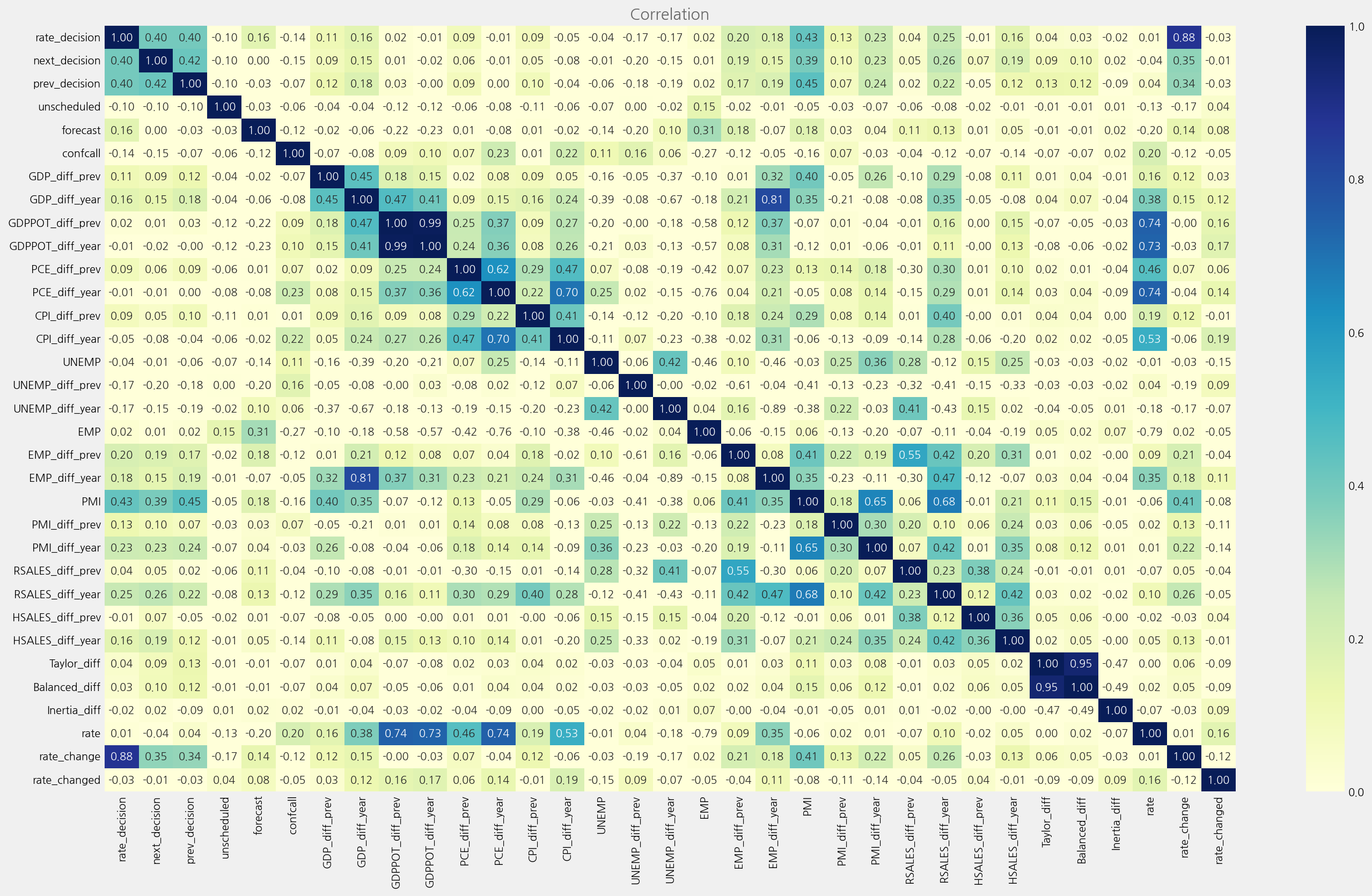
Observation on the correlation:
Higher correlation with Rate Decision:
‘GDP_diff_year’
‘Unemp_diff_prev’
‘Employ_diff_prev’
‘PMI’
‘RSALES_diff_year’
‘HSALES_diff_year’
‘prev_decision’
Will create two dataset, one full set and the other smaller set with high correlation
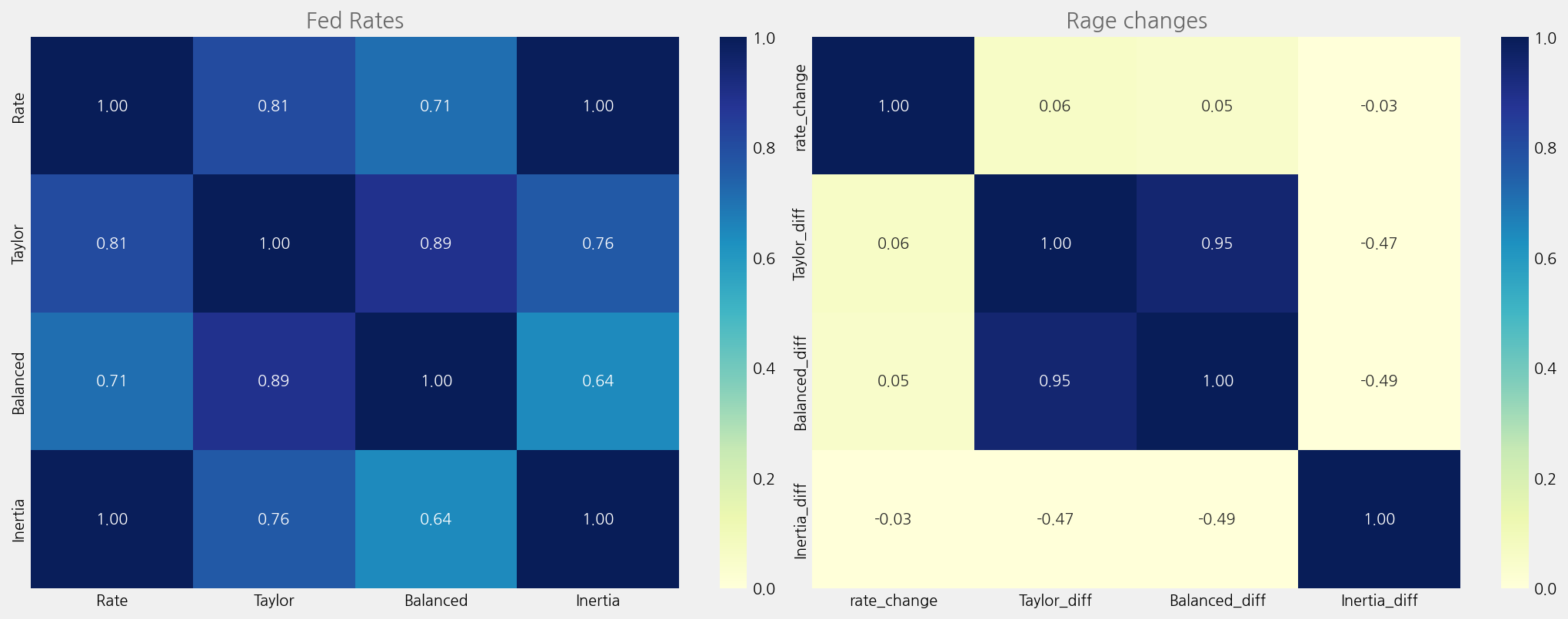
Correlation between Taylor rule and actual rates#
corr_columns = ["Rate", "Taylor", "Balanced", "Inertia"]
corr_data1 = econ_data[corr_columns].astype(float).corr()
corr_columns = ["rate_change", "Taylor_diff", "Balanced_diff", "Inertia_diff"]
corr_data2 = econ_data[corr_columns].astype(float).corr()
cfg = eKonf.compose("visualize/plot=heatmap")
cfg.figure.figsize = (15, 6)
cfg.subplots.ncols = 2
cfg.subplots.nrows = 1
cfg.heatmap.axno = 0
cfg.heatmap.datano = 0
cfg.heatmap.cmap = "YlGnBu"
cfg.heatmap.vmin = 0
cfg.heatmap.vmax = 1
cfg.heatmap.fmt = ".2f"
cfg.ax.title = "Fed Rates"
cfg.ax.axno = 0
heatmap2 = cfg.heatmap.copy()
heatmap2.axno = 1
heatmap2.datano = 1
ax2 = cfg.ax.copy()
ax2.title = "Rage changes"
ax2.axno = 1
cfg.plots.append(heatmap2)
cfg.axes.append(ax2)
eKonf.instantiate(cfg, data=[corr_data1, corr_data2])
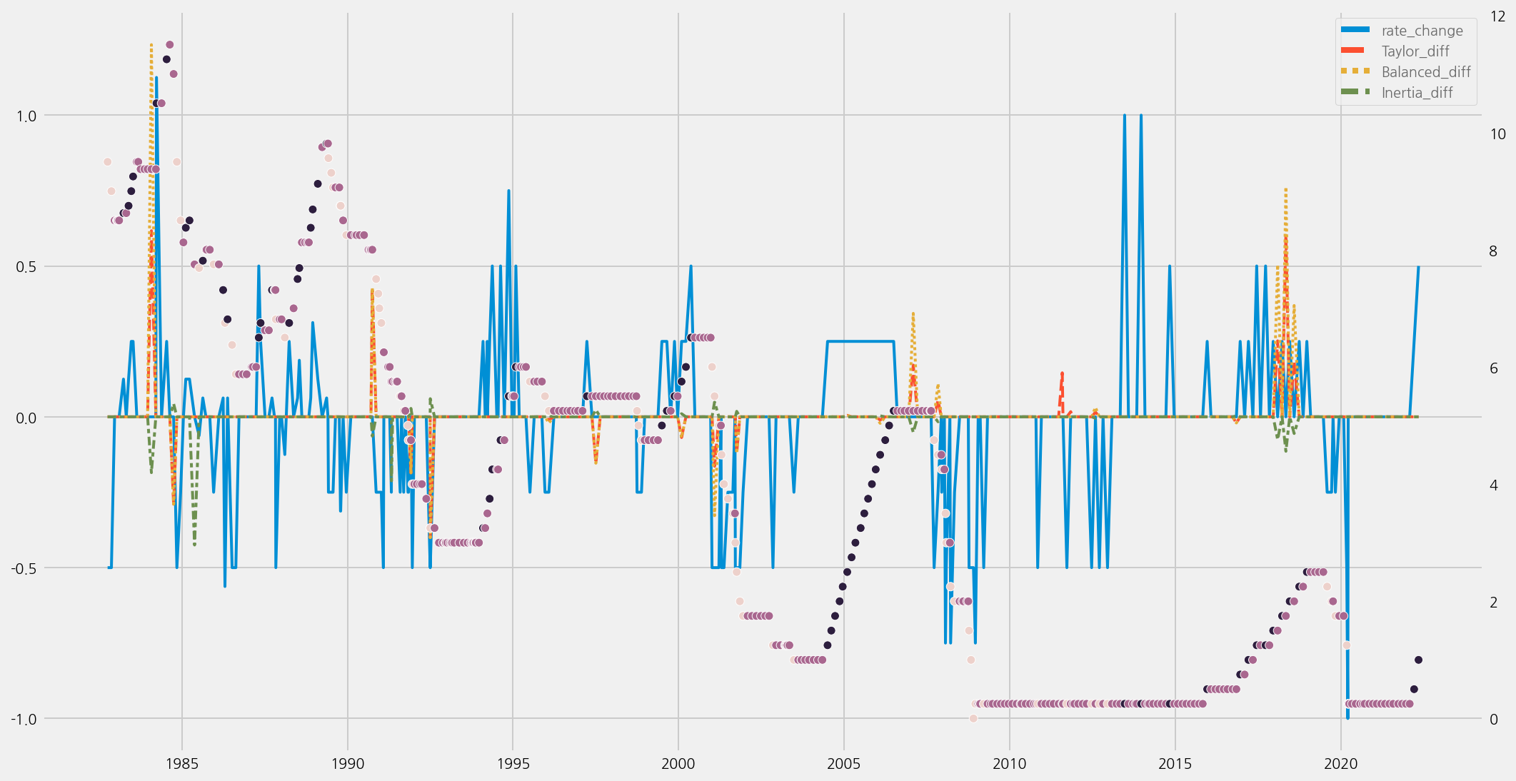
cfg = eKonf.compose("visualize/plot=lineplot")
cfg.figure.figsize = (15, 8)
cfg.lineplot.y = corr_columns

scatter_cfg = eKonf.compose("visualize/plot/scatterplot")
scatter_cfg.x = "date"
scatter_cfg.y = "rate"
scatter_cfg.hue = "rate_decision"
scatter_cfg.secondary_y = True
cfg.plots.append(scatter_cfg)

ax2 = cfg.ax.copy()
ax2.grid = False
ax2.secondary_y = True
cfg.axes.append(ax2)

eKonf.instantiate(cfg, data=econ_data)