N-grams for Tokenization#
N-grams are a crucial concept in the field of Natural Language Processing (NLP) and are extensively used in text processing and modeling. They represent a sequence of ‘n’ items in a given sample of text or speech. Let’s break down this concept and learn how to apply it for tokenization.
Understanding N-grams#
N-grams are contiguous sequences of n items in a text. When applied to text, an item could be a character, a word, or a sentence. For instance, in the sentence “I love dogs”, the 1-grams (also known as unigrams) are “I”, “love”, “dogs”, the 2-grams (bigrams) are “I love”, “love dogs”, and the only 3-gram (trigram) is “I love dogs”.
The ‘n’ in n-gram stands for the number of grouped words. Therefore, a 1-gram is a single word, a 2-gram consists of two words, a 3-gram consists of three words, and so on.
Why use N-grams?#
One of the primary uses of n-grams in NLP is to capture the language structure, such as phrases and other commonly occurring word sequences. This not only helps us understand the context better but also assists in predicting the next item in a sequence, which is highly beneficial in language modeling, spelling correction, and even speech recognition.
N-grams in Tokenization#
Tokenization is the process of splitting a large paragraph into sentences or words. When we apply the concept of n-grams in tokenization, we divide the text into chunks of n contiguous items (usually words). Each chunk (or token) can then be analyzed separately. This is particularly useful when the context between words is necessary to better understand the meaning of the text.
For instance, in the phrase “New York”, treating “New” and “York” as separate tokens (unigrams) loses the meaning that the two words together represent a single entity (a city). But if we treat “New York” as a single token (a bigram), we can preserve this meaning.
Here is an example of how to implement tokenization using n-grams:
import nltk
from nltk.util import ngrams

text = "I love to play football."
tokenized_text = nltk.word_tokenize(text)
bigrams = list(ngrams(tokenized_text, 2))
print(bigrams)
Output:
[('I', 'love'), ('love', 'to'), ('to', 'play'), ('play', 'football.')]
In the example above, we first tokenize the input text into individual words using nltk.word_tokenize(). We then generate the bigrams using the ngrams() function.
N-grams, Dimensionality, and Managing Vocabulary#
As we generate n-grams for larger values of ‘n’, we will see a significant increase in the number of features. This increase can lead to a high-dimensional feature space and cause computational challenges due to the curse of dimensionality. Therefore, it’s essential to manage the feature space effectively.
High Dimensionality in N-grams#
For example, considering a corpus with 1,000 unique words:
If we use 1-grams (unigrams), we get 1,000 features
For 2-grams (bigrams), we can have up to 1,000 * 1,000 = 1,000,000 features.
This exponential increase poses problems in terms of memory and computational efficiency. It is essential to filter out low-frequency and uninformative n-grams to keep the feature space manageable.
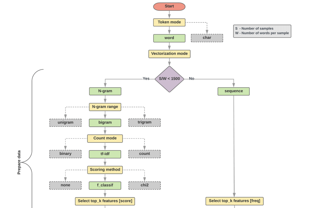
Fig. 78 Text classification flowchart (from Google Developers)#
Hashing Vectorizer#
One way to deal with high-dimensional feature spaces is to use a Hashing Vectorizer. Instead of mapping each n-gram to a unique integer in our feature space (as CountVectorizer does), a Hashing Vectorizer hashes the n-grams into a fixed number of buckets. This is a lossy transformation (some information is lost), but it can help maintain a manageable feature space.
The hash function used in the vectorizer is deterministic, which means that it will always map the same n-gram to the same integer.
Here’s an example of how to use a Hashing Vectorizer:
from sklearn.feature_extraction.text import HashingVectorizer

vectorizer = HashingVectorizer(
    n_features=2**4, stop_words="english", alternate_sign=False
)

X = vectorizer.transform(corpus)

print(X.shape)
In the code snippet above, we transform our text data into a feature matrix with a fixed size of 16 (2**4) using the HashingVectorizer.
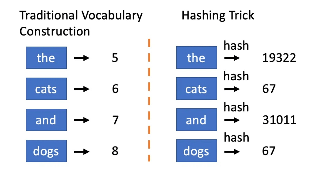
Fig. 79 Hashing Vectorizer#
Collocations#
Another essential concept in NLP is Collocations, which are phrases that occur together more often than would be expected by chance. These phrases can be non-compositional (their meaning is not just the sum of their parts), non-substitutable (you can’t substitute a part with its synonym), and non-modifiable (you can’t modify the phrase with additional words).
Non-compositional: meaning is not the sum of its parts
e.g., “New York” is not the sum of “New” and “York”
Non-substitutable: cannot substitute with a synonym
e.g., “fast food” is not the same as “quick food”
Non-modifiable: cannot modify with additional words
e.g., “kick around the bucket” is not the same as “kick the bucket around”
Pointwise Mutual Information#
Pointwise Mutual Information (PMI) is a measure of how often two words co-occur in a corpus, considering their individual probabilities. PMI helps rank word pairs based on how often they collocate, compared to how often they would theoretically collocate if they were independent.
PMI of two words \(w_1\) and \(w_2\) is defined as:
where \(w_1\) and \(w_2\) are words in the vocabulary, and \(w_1\), \(w_2\) is the N-gram \(w_1\_w_2\). ranks words by how often they collocate, relative to how often they occur apart.
It can be generalized to n-grams as:
Caveat: PMI is biased towards rare words. It is more likely to overestimate the strength of association between two rare words than between two frequent words. This is because the denominator of the PMI equation is the product of the individual probabilities of the words, which is smaller for rare words.
Out-of-Vocabulary Words (OOV) for N-grams#
In any text analysis, we often encounter words that are not in our predefined vocabulary, also known as out-of-vocabulary (OOV) words. This is especially true for n-gram models, where the number of potential word sequences can be enormous.
There are several strategies for dealing with OOV words:
Replace them with a special token, e.g.,
<UNK>.Replace them with their part-of-speech tag, e.g.,
<NOUN>.Replace them with a higher-level category or hypernym, e.g.,
<ANIMAL>.Use a hash function to map OOV words to a fixed number of buckets, similar to the hashing trick mentioned above.
These strategies can help manage the vocabulary and keep the feature space manageable while dealing with new or unexpected words in the data.