Word Embeddings#

What are word embeddings?#
Word embeddings are a captivating facet of natural language processing that enable us to represent words as vectors. These vectors, learned from the textual data, encapsulate much of the semantic and syntactic properties of words, enabling us to quantify and analyze linguistic relationships with mathematical precision.
Picture two sentences: “The cat is lying on the floor and the dog was eating,” and “The dog was lying on the floor and the cat was eating.” Despite the switched roles of ‘cat’ and ‘dog’ in these sentences, we instinctively comprehend their similarity - they are both common pets and lovable internet sensations. Word embeddings capture this similarity by assigning similar vector representations to the words ‘cat’ and ‘dog’.
But how does this work exactly? Essentially, a word embedding is a function that is parameterized by a vector of real numbers, denoted as 𝜃. When this function is applied to a word w, it yields the vector 𝜃 - the embedding of the word w. In simpler words, every word is transformed into a corresponding vector of real numbers that encapsulates its ‘meaning’ in the multi-dimensional vector space.
The concept of ‘embedding’ extends beyond the realm of NLP. More broadly, it denotes the process of representing a high-dimensional object - like a document in NLP or an image in computer vision - as a lower-dimensional, dense vector. The power of embeddings lies in their ability to condense a vast amount of information into a compact, manageable form without losing the core essence of the original object.
While word embeddings like word2vec, GloVe, BERT, and ELMo have made a name for themselves in the NLP world, it’s important to distinguish that not all representations of words qualify as embeddings. Methods like one-hot encoding, bag-of-words, and TF-IDF, for instance, are not deemed as embeddings. These techniques, along with tools like sklearn’s CountVectorizer count vectors or counts over LIWC dictionary categories, represent words in a way that lacks the dense, continuous, and comparative nature of word embeddings. Conversely, PCA reductions of word count vectors, LDA topic shares, and compressed encodings from an autoencoder are considered embeddings, thanks to their capacity to capture the contextual and semantic richness of the data they represent.
In a nutshell, word embeddings are an incredible tool that allows us to project the vast landscape of human language onto the precise terrain of mathematics, facilitating the analysis, understanding, and manipulation of words in ways previously unimagined.
Categorical Embeddings#
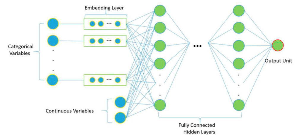
Fig. 87 Categorical Embeddings#
Categorical embeddings offer a powerful way to represent categorical variables, which are common in various fields like market research, medical studies, and social science, as vectors. This method is especially beneficial when dealing with high-dimensional categorical variables - variables that have a large number of categories.
Imagine a binary classification problem where the outcome is denoted by \(Y\), and you’re dealing with a high-dimensional categorical variable \(X\) that has 1000 categories. Naturally, the first instinct might be to represent \(X\) as a vector of length 1000. However, the challenge here is that it becomes computationally intensive for a machine learning model to learn from such a high-dimensional categorical variable.
This is where categorical embeddings come to the rescue. Instead of representing \(X\) as a high-dimensional vector, we can represent it as a lower-dimensional vector of length \(k\) (for instance, 10). This process effectively transforms \(X\) into a manageable and useful form without losing its core information - the essence of what embeddings are all about.
There are primarily two approaches to creating categorical embeddings:
Principal Component Analysis (PCA): The first approach applies PCA, a dimensionality reduction technique, to the dummy variables \(X\) to create a lower-dimensional vector representation, denoted by \(\tilde{X}\). This compressed representation of \(X\) enables models to work more efficiently while preserving the variance in the data.
Regression Prediction: The second approach involves regressing \(Y\) on \(X\), predicting \(\hat{Y}(X_i)\), and then using this prediction as a feature in a new model. Essentially, it leverages the prediction from one model as a feature for another, creating a richer representation of the original categorical variable.
In essence, categorical embeddings are an elegant solution to a complex problem, simplifying high-dimensional categorical data into a compact form, allowing machine learning models to learn more effectively and efficiently.
An embedding layer is matrix multiplication:#
An embedding layer in neural networks is essentially a matrix multiplication operation. To understand this, consider the following formula:
Here, \(x\) represents a categorical variable, such as a word. This variable is encoded as a one-hot vector, with a single item equating to one. \(x\) acts as the input to the embedding layer.
On the other hand, \(h_1\) denotes the first hidden layer of the neural network, which is the output of the embedding layer.
What links \(x\) and \(h_1\) is the embedding matrix, denoted as \(\omega_E\). This matrix encodes predictive information about the categories, transforming the input into the output.
But the embedding matrix is not merely a mathematical tool; it has a rich spatial interpretation when projected into 2D space. Each row of \(\omega_E\) serves as a vector in \(n_E\)-dimensional space. Hence, the rows of \(\omega_E\) can be viewed as the coordinates of points in this vector space, where each point represents a category.
This spatial representation illuminates the relationships between categories in a powerful way:
The distance between points in the space is indicative of the similarity between the corresponding categories. Categories that are closer together are more similar.
The angle between points in the space can be seen as the relationship between the corresponding categories. Categories with smaller angles between them are more closely related.
In this way, an embedding layer elegantly transforms categorical data into a format that neural networks can work with effectively while preserving the intricate relationships between categories.
Embedding Layers vs. Dense Layers#
When it comes to neural networks, there’s a fascinating relationship between embedding layers and dense layers. In fact, an embedding layer can be seen as statistically equivalent to a fully-connected dense layer, provided we have one-hot vectors as input and a linear activation function.
Here’s why: an embedding layer takes a one-hot encoded vector, multiplies it by the embedding matrix (which is just a learned look-up table), and produces an output. This is essentially what a dense layer with a linear activation does too. In a dense layer, the input is multiplied by the weights (equivalent to the embedding matrix in an embedding layer), and an optional bias is added. If we don’t use a bias and the activation is linear, then the dense layer does exactly the same as the embedding layer.
However, while functionally similar, an important distinction between the two lies in their efficiency. Specifically, embedding layers are much faster than dense layers when dealing with a large number of categories (generally more than around 50). The reason for this speed difference is the computational expense involved in matrix multiplication. In an embedding layer, the matrix multiplication with a one-hot encoded vector effectively boils down to selecting the corresponding row in the embedding matrix, which is a much simpler operation.
In contrast, a dense layer with a one-hot vector as input would still perform a full matrix multiplication, which is more computationally expensive. So, while both layers can theoretically perform the same operation, when it comes to handling a high number of categories, the embedding layer stands out as the more efficient choice.
Word Embeddings#
Word embeddings are an innovative application of neural network layers. They provide an efficient, dense representation for words by mapping them onto vectors.
Here’s how they work: Consider any document, which we can view as a list of word indexes, \({w_1 ,w_2 ,...,w_{n_i} }\). Each \(w_i\) can be represented as a one-hot vector. The dimensionality of this vector, \(n_w\), equals the size of the vocabulary - each word in the vocabulary has a unique index that is marked as ‘1’ in the one-hot vector, while all other indexes are ‘0’.
To ensure consistent input structure for the neural network, it is usually necessary to normalize all documents to the same length, \(L\). This can be done by padding shorter documents with a null token. However, it’s worth noting that this requirement can be relaxed when using recurrent neural networks.
The magic happens in the embedding layer. This layer replaces the sparse one-hot vectors with a list of dense vectors. Each dense vector \(x_j\) has a lower dimensionality \(n_E\) (where \(n_E\) << \(n_w\) ). The embedding layer produces an array \(\mathbf{X}\) of these dense vectors:
How is each \(x_j\) produced? It’s done via matrix multiplication between the embedding matrix \(\mathbf{E}\) and the one-hot vector \(w_j\):
The embedding matrix \(\mathbf{E}\) contains the word vectors. Each column in this matrix is associated with a word from the vocabulary. The dot product with the one-hot vector \(w_j\) selects the column (i.e., the word vector) associated with the word at index \(j\).
After this transformation, \(\mathbf{X}\) is then flattened into a single \(L * n_E\) vector which serves as input to the next layer of the neural network.
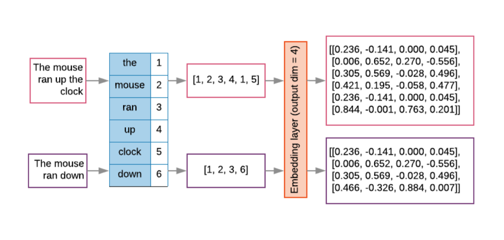
Fig. 88 Word Embeddings#
In a nutshell, word embeddings offer an efficient, computationally friendly way of representing words for machine learning tasks, condensing the high-dimensional space of one-hot vectors into a denser, lower-dimensional representation that still captures essential semantic features.
Why do we need neural networks for word embeddings?#
In the realm of machine learning and natural language processing, we often face a dilemma when dealing with text data: should we use traditional clustering algorithms, or do we need the more advanced neural network models for tasks such as word embeddings?
There’s a good number of conventional, or as we often call them, shallow algorithms, that work remarkably well for clustering tasks. These include:
k-means clustering: An algorithm that groups similar data points into ‘k’ number of clusters.
Hierarchical clustering: A method that builds nested clusters by merging or splitting them successively.
Spectral clustering: An approach that uses eigenvalues (the ‘spectrum’) of a similarity matrix to reduce the dimensionality of the data before clustering in fewer dimensions.
PCA (Principal Component Analysis): A technique that helps identify the most significant variables and eliminate redundant ones.
Despite the effectiveness of these methods, we frequently turn to neural networks for generating word embeddings. Why so? Here are the compelling reasons:
Learning Relationships: Unlike shallow algorithms, neural networks can learn and capture the relationships between words based on their contexts in the corpus. This is an essential aspect of semantic understanding in natural language processing.
Useful for Downstream Tasks: The word embeddings produced by neural networks can be readily used as input to downstream tasks such as text classification, sentiment analysis, or machine translation.
Mapping Discrete Words to Continuous Vectors: Neural networks facilitate a continuous, dense representation for words that was otherwise sparse and high-dimensional in one-hot encoded format. This condensed representation is what we refer to as word embeddings.
Solution to the Curse of Dimensionality: Lastly, word embeddings generated by neural networks effectively tackle the ‘curse of dimensionality’. This refers to the challenge posed by extremely high-dimensional data (like text data) that becomes increasingly sparse, and hence difficult for many machine learning algorithms to handle.
In conclusion, while traditional clustering algorithms hold their merits in specific scenarios, the flexibility, learning ability, and higher representation power of neural networks make them the go-to choice for tasks such as word embeddings in natural language processing.