Topic Coherence Measures#

Introduction#
Topic coherence represents the overall interpretability of topics and is used to assess their quality. It is essential in topic modeling, a technique that aims to explain a collection of documents as a mixture of topics. Evaluating topics based on their interpretability is necessary, as mathematically optimal topics are not always human-readable. Topic coherence is a measure of interpretability and is used to evaluate the quality of topics. It tries to represent the degree of semantic similarity between high scoring words in a topic.
Topic Modeling#
Topic modeling aims to explain a collection of documents as a mixture of topics, where each topic is a distribution over words, and each document is a distribution over topics. The goal of topic modeling is to find the topics and their distributions over words and documents. The assumption behind topic modeling is that:
A text (document) is composed of several topics.
A topic is composed of several words.
Evaluating Topics#
Evaluating topics using topic coherence is essential for determining the quality and interpretability of the topics generated by topic modeling algorithms. Let’s take a look at a few simple examples to better understand this concept.
Suppose a topic modeling algorithm has generated the following topics from a given document collection:
Topic 1:
['coffee', 'espresso', 'cappuccino', 'latte']Topic 2:
['gardening', 'plants', 'flowers', 'soil']Topic 3:
['house', 'red', 'building', 'green']
In these examples, Topic 1 and Topic 2 seem to be coherent and easily interpretable because the words within each topic are closely related semantically. Topic 1 is related to different types of coffee, while Topic 2 is about gardening and plants.
However, Topic 3 is less coherent and harder to interpret. Although ‘house’ and ‘building’ are related, the words ‘red’ and ‘green’ do not seem to fit well within the topic. The lack of coherence in Topic 3 could indicate that the topic modeling algorithm might need further tuning or that the document collection might contain some noise.
Using topic coherence measures, we can quantify the coherence of each topic and compare them. High coherence scores would indicate that the topics are easily interpretable and semantically related, whereas low coherence scores would signify that the topics are less interpretable and might require further investigation.
Topic Coherence#
Topic coherence assesses how well a topic is supported by a text corpus. It uses statistics and probabilities drawn from the text corpus to measure the coherence of a topic, focusing on the word’s context. Topic coherence depends on both the words in a topic and the reference corpus.
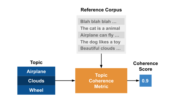
Fig. 51 Topic Coherence#
A general structure for topic coherence measures has been proposed by Röder, M. et al [Röder et al., 2015]. It consists of three components:
Segmentation
Probability Calculation
Confirmation Measure
Aggregation
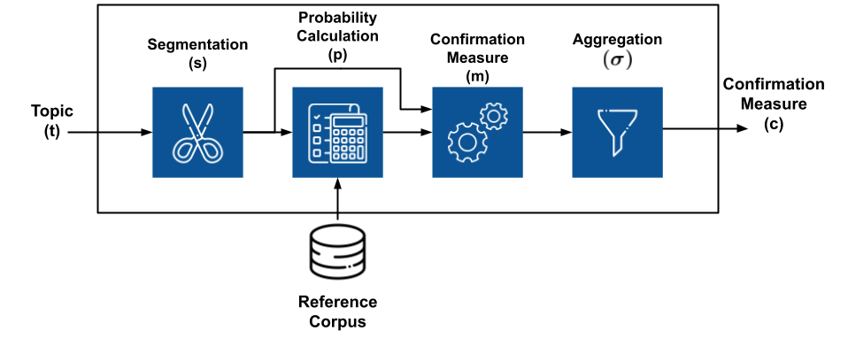
Fig. 52 Topic Coherence Structure#
1. Segmentation#
The segmentation module is a crucial step in the coherence measurement process, as it creates pairs of word subsets used to assess the coherence of a topic. Given a topic \(t\) represented by its top-n most important words \(W = \{w_1, w_2, \dots, w_n\}\), the application of a segmentation \(S\) results in a set of subset pairs derived from \(W\):
Segmentation can be understood as the method we use to combine words in a topic before evaluating their relationships.
For instance, the S-one-one segmentation requires the creation of pairs of distinct words. If \(W = \{w_1, w_2, \dots, w_n\}\), then the S-one-one segmentation generates the following pairs:
By using this approach, our model computes the final coherence score based on the relationship between each word in the topic and the other words in the topic.
Another example is the S-one-all segmentation, which entails creating pairs of each word with all other words. Applying it to \(W\) yields the following pairs:
By using this approach, our model computes the final coherence score based on the relationship between each word in the topic and all the other words in the topic. This way, the segmentation step allows us to choose different strategies to investigate the coherence of a given topic.
2. Probability Calculation#
The probability calculation module is a crucial component in coherence metrics, as it computes the probabilities for word subsets generated by the segmentation module. These probabilities are derived from the textual corpus and are essential for understanding the relationships between words in a topic.
For instance, we might be interested in calculating the following probabilities:
\(P(w)\): the probability of a word \(w\) occurring in the corpus.
\(P(w_1, w_2)\): the probability of a word pair \((w_1, w_2)\) occurring in the corpus.
Various techniques can estimate these probabilities in distinct ways. One example is the estimation of \(P_{bd}(w)\), which is calculated by counting the number of documents containing the word \(w\) and dividing it by the total number of documents in the corpus:
Similarly, the probability \(P(w_1, w_2)\) can be estimated by counting the number of documents in which both \(w_1\) and \(w_2\) appear and dividing the result by the total number of documents in the corpus:
Another approach is to use sentence-level probabilities. In this case, the probability \(P_{bs}(w)\) is calculated by counting the number of sentences in which the word \(w\) appears and dividing the result by the total number of sentences in the corpus.
Alternatively, for \(P_{sw}\), the probability is determined by counting the number of sliding windows containing the word \(w\) and dividing the result by the total number of sliding windows in the corpus.
These probabilities serve as the foundation for computing coherence metrics and are essential for evaluating the quality of topics generated by topic modeling algorithms.
3. Confirmation Measure#
The confirmation measure module lies at the heart of coherence metrics, as it calculates the confirmation of word subsets. It assesses how well a word subset \(W^*\) supports the words in another subset \(W^{\prime}\) by comparing their probabilities derived from the textual corpus.
The confirmation measure aims to evaluate the relationship between two subsets of words by analyzing how likely they are to appear together in the corpus. If the words in \(W^{\prime}\) frequently co-occur with those in \(W^*\), the confirmation measure will be high; if not, it will be low.
For instance, suppose we have the following word subsets:
\(W^{\prime} = \{w_1, w_2\}\)
\(W^* = \{w_3, w_4\}\)
A high confirmation measure indicates that the words \(w_1\) and \(w_2\) are likely to appear with the words \(w_3\) and \(w_4\) in the reference corpus.
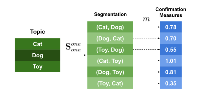
Fig. 53 Confirmation Measures#
Confirmation measures can be classified into two types: direct and indirect.
Direct Confirmation Measure#
The direct confirmation measure is a straightforward approach that compares the probabilities of word subsets \(W^{\prime}\) and \(W^*\).
Alternatively, using logarithms:
Here, \(\epsilon\) represents a small constant that prevents undefined values for logarithms.
Indirect Confirmation Measure#
The indirect confirmation measure is a more sophisticated method. It computes a direct confirmation measure for each word in the subsets \(W^{\prime}\) and \(W^*\), producing a vector of confirmation scores for each word in \(W^{\prime}\).
where \(|W|\) denotes the number of words in \(W\).
The process is repeated for the subset \(W^*\). The indirect confirmation measure is then the similarity between the two vectors.
In this case, \(sim\) is a similarity function, such as cosine similarity.
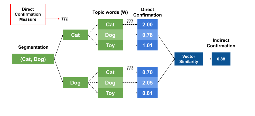
Fig. 54 Indirect Confirmation Measures#
The indirect confirmation measure captures relationships that the direct confirmation measure might overlook. For example, while the words ‘cats’ and ‘dogs’ may never appear together in the dataset, they could frequently co-occur with the words ‘toys’, ‘pets’, and ‘cute’. The direct confirmation measure would fail to identify the relationship between ‘cats’ and ‘dogs’ since they never appear together. However, the indirect confirmation measure would detect this relationship by observing that ‘cats’ and ‘dogs’ frequently appear with the words ‘toys’, ‘pets’, and ‘cute’.
Aggregation#
The aggregation module plays a crucial role in computing the final coherence score for a topic. It aggregates the confirmation scores of the pairs generated in the previous steps, condensing the information into a single value that represents the topic’s coherence.
Various aggregation techniques can be employed, including mean, median, and geometric mean, among others. Each method has its advantages and disadvantages, and the choice of aggregation technique depends on the specific use case and the desired properties of the resulting coherence score.
Mean#
The mean (arithmetic average) is a widely-used aggregation technique. It calculates the sum of the confirmation scores and divides it by the total number of scores. The mean is sensitive to extreme values and might not be the best choice if the distribution of scores is skewed.
Median#
The median represents the middle value in a sorted list of confirmation scores. It is less sensitive to extreme values compared to the mean and provides a more robust estimate of central tendency, especially in cases where the distribution of scores is not symmetrical.
Geometric Mean#
The geometric mean is another aggregation technique that calculates the nth root of the product of confirmation scores, where n is the total number of scores. The geometric mean is less sensitive to extreme values than the mean and is particularly useful when dealing with multiplicative factors or when the data has a log-normal distribution.
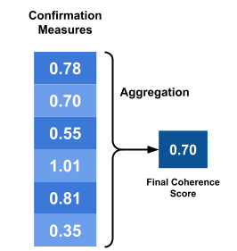
Fig. 55 Aggregation Techniques#
In summary, the aggregation module is responsible for combining the confirmation scores of word subset pairs into a single coherence score that represents the topic’s interpretability. The choice of aggregation technique depends on the desired properties of the coherence score and the distribution of confirmation scores.
Putting Everything Together#
To measure the coherence of a topic, the following steps are taken:
Topic Selection: Identify the topic \(T\) for which you want to measure coherence.
Reference Corpus: Choose a reference corpus \(C\) that represents the context of the topic.
Top-n Words Extraction: Extract the top-n most important words in the topic \(T\), resulting in a word subset \(W\).
Segmentation: Segment the word subset \(W\) into pairs of words, generating a set of word subsets \(S\).
Probability Calculation: Utilize the reference corpus \(C\) to calculate the probabilities of the word subsets \(S\).
Confirmation Measure: Compute the confirmation measure for each pair of words in \(S\) using the probabilities obtained from the reference corpus \(C\).
Aggregation: Aggregate all the confirmation scores into a single coherence score for the topic \(T\).
If you have multiple topics, repeat the process for each topic and use the average coherence score as a measure of the overall quality of the topic model.
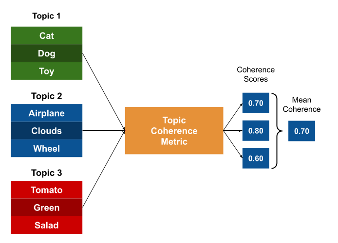
Fig. 56 Coherence Score for Multiple Topics#
The Gensim library offers a class that implements four widely-used coherence models: \(u_{mass}\), \(c_v\), \(c_{uci}\), and \(c_{npmi}\).
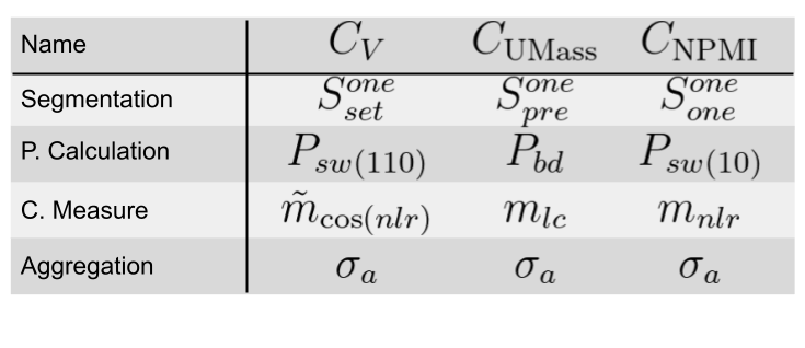
Fig. 57 Gensim Coherence Models#
The \(C_{NPMI}\) coherence model uses the following steps:
Segmentation: S-one-one (one word in each subset)
Probability estimation: probabilities are calculated using a sliding window of size 10.
Confirmation measure: Normalized Pointwise Mutual Information (NPMI) is employed.
The \(C_V\) coherence model involves these steps:
Segmentation: S-one-set, where the confirmation measure is calculated for pairs of words in the same subset.
Probability estimation: probabilities are calculated using a sliding window of size 110.
Confirmation measure: indirect confirmation measure with cosine similarity as the similarity function.
Aggregation: the mean of the confirmation scores is used for aggregation.
In summary, measuring topic coherence involves a series of steps, from selecting a topic and reference corpus to calculating probabilities, confirmation measures, and aggregating scores. These steps help assess the interpretability and quality of a topic model, providing valuable insights for users.
Understanding Pointwise Mutual Information#
Determining whether two (or more) words are related or form a concept can be achieved by assessing their co-occurrence patterns:
If words appear together more often than expected by chance, it suggests they are related.
However, caution is needed, as some words may co-occur frequently just because they are common. For instance, in the case of “New York,” the word “New” frequently appears in news articles, so it may co-occur with other words more often than expected by chance.
To discern whether the co-occurrence of “New” and “York” is due to chance or an actual relationship, a measure like Pointwise Mutual Information (PMI) can be employed.
PMI is used to determine the association between two words, quantifying the likelihood of their co-occurrence in text given their individual appearances.
PMI#
PMI is defined as:
Here, \(P(w_i, w_j)\) denotes the probability of words \(w_i\) and \(w_j\) appearing together in the corpus, while \(P(w_i)\) and \(P(w_j)\) represent the probabilities of \(w_i\) and \(w_j\) occurring individually.
If \(w_i\) and \(w_j\) are independent, \(P(w_i, w_j) = P(w_i)P(w_j)\), and the PMI equals zero.
If \(w_i\) and \(w_j\) are dependent, \(P(w_i, w_j) > P(w_i)P(w_j)\), and the PMI is positive.
If \(w_i\) and \(w_j\) are negatively dependent, \(P(w_i, w_j) < P(w_i)P(w_j)\), and the PMI is negative.
Normalized Pointwise Mutual Information#
While PMI effectively measures the association between two words, it has some limitations. For example, PMI is not normalized, making it difficult to compare associations between words with different frequencies.
Normalized Pointwise Mutual Information (NPMI) addresses this issue by normalizing PMI. It is defined as:
In summary, understanding the association between words using PMI or NPMI helps determine whether they form a concept or are related. By considering the co-occurrence patterns of words and their individual frequencies, these measures provide valuable insights into the relationships between words in a corpus.
Understanding Cosine Similarity#
Cosine similarity is a measure used to determine the similarity between two vectors. It assesses the cosine of the angle between the vectors, which provides a measure of similarity that is independent of their magnitude. The formula for cosine similarity is:
Here, \(A\) and \(B\) represent the two vectors being compared, and \(\theta\) is the angle between them.
Cosine similarity produces a value between -1 and 1:
If the two vectors are identical, the cosine similarity is 1.
If the two vectors are orthogonal (i.e., not related), the cosine similarity is 0.
If the two vectors are antipodal (i.e., opposite directions), the cosine similarity is -1.
If the two vectors are similar (i.e., pointing in the same direction), the cosine similarity is positive.
If the two vectors are dissimilar (i.e., pointing in different directions), the cosine similarity is negative.
In the context of natural language processing and information retrieval, cosine similarity is often used to measure the similarity between documents or between a query and a document. In this scenario, each document or query is represented as a high-dimensional vector, where each dimension corresponds to a specific term in the vocabulary, and the value of each dimension represents the weight (e.g., term frequency) of that term in the document.
By computing the cosine similarity between these vectors, it is possible to identify documents or queries with similar semantic content, even if they do not share the exact same words. This is because the cosine similarity focuses on the direction of the vectors, which is influenced by the overall distribution of terms, rather than the specific words themselves.