Word Similarity

In the field of Natural Language Processing (NLP), understanding the semantics or the meaning of words is crucial. To achieve this, NLP uses context in two primary ways:

1. Distributional similarity (also known as vector-space semantics): This approach assumes that words occurring in similar contexts tend to have similar meanings. The set of all contexts in which a word appears is used to measure the similarity between words.

2. Word sense disambiguation: This approach is based on the assumption that if a word has multiple meanings, then it would occur in different contexts for each meaning. The context of a particular occurrence of a word is used to identify the ‘sense’ or meaning of the word in that context.

Distributional Similarity

The basic idea of distributional similarity is to measure the semantic similarities of words by measuring the similarity of their contexts. This is achieved by representing words as sparse vectors where:

• Each vector element (or dimension) represents a different context.

• The value of each element is the frequency of the context in which the word occurs, capturing how strongly the word is associated with that context.

• The semantic similarity of words is then computed by measuring the similarity of their context vectors.

The concept of distributional similarity can be better understood from an Information Retrieval perspective where we search a collection of documents for specific terms.

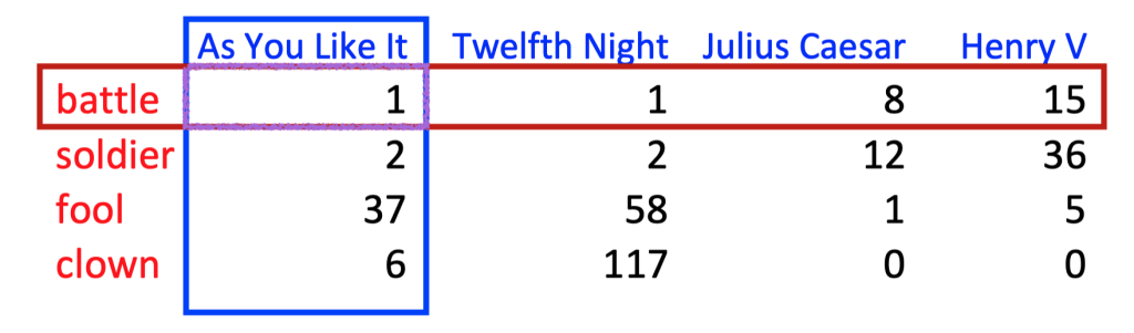
Fig. 80 Term-Document Matrix

Here, we have a term-document matrix, which is a two-dimensional matrix:

• Each row represents a term in the vocabulary.

• Each column represents a document.

• Each element is the frequency of the term in the document.

In this representation, each document is a column vector, where each entry represents the frequency of a term in the document. Similarly, each term is a row vector, with each entry representing the frequency of the term in a document. Two documents (or two words) are similar if their vectors are similar.

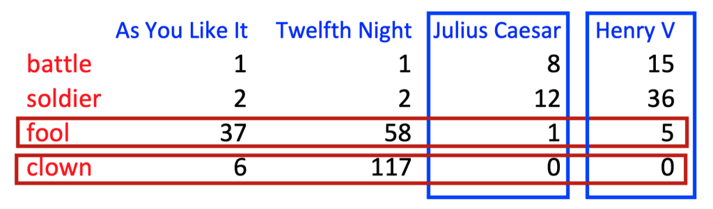
Fig. 81 Similar Documents in Term-Document Matrix

This matrix can be used to implement a model of the distributional hypothesis if we treat each context as a column and each word as a row.

What is a ‘context’?

The definition of a context can vary based on the requirements:

• Contexts defined by nearby words: How often does a word occur within a window of a certain number of words of another word, or in the same document or sentence? This yields broad thematic similarities between words.

• Contexts defined by grammatical relations: How often does a word occur as the subject of another word? This requires a grammatical parser to identify the grammatical relations between words and yields more fine-grained similarities between words.

For example, we can represent words using a fixed vocabulary of context words and count the number of times each context word occurs within a window of words.

Word-Word Matrix

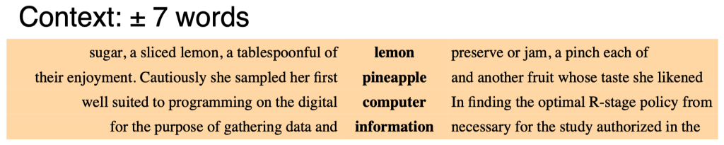
Fig. 82 Word-Word Matrix

In a word-word matrix, we count the co-occurrences of words within a defined context. The context can be defined in various ways such as:

• Within a fixed window: How often does a context word occur within a fixed number of words around the target word?

• Within the same sentence: How often do the target and context words occur in the same sentence?

• By grammatical relations: How often does a context word occur in a certain grammatical relation with the target word?

Depending on the information we want to capture, we can represent co-occurrences as binary features (does/doesn’t occur), as frequencies (how often it occurs), or as probabilities (the probability of occurrence).

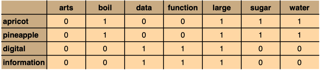
Fig. 83 Co-occurrence as binary features

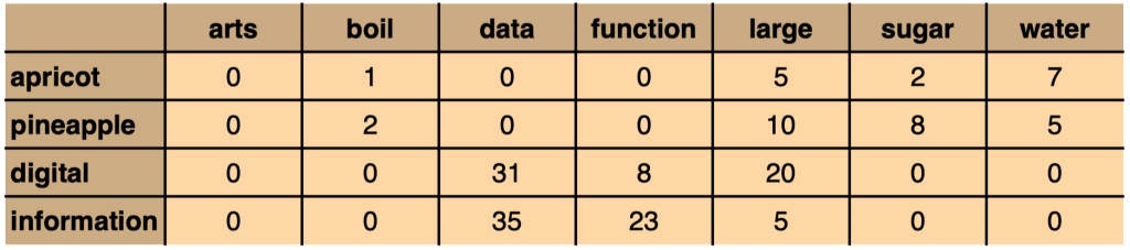
Fig. 84 Co-occurrence as frequencies

Dot Product as Similarity

When the vectors consist of simple binary features (0,1), the dot product can be used as a similarity metric:

\[ sim_{dot-prod}(\vec{x}\cdot\vec{y}) = \sum_{i=1}^{N} x_i \times y_i \]

However, the dot product isn’t a good metric if the vector elements are arbitrary features, as it prefers long vectors. This is where the cosine similarity comes in.

Vector Similarity: Cosine

One way to define the similarity of two vectors is to use the cosine of their angle. The cosine of two vectors is their dot product, divided by the product of their lengths:

\[ sim_{cos}(\vec{x},\vec{y})=\frac{\sum_{i=1}^{N} x_i \times y_i}{\sqrt{\sum_{i=1}^{N}x_i^2}\sqrt{\sum_{i=1}^{N}y_i^2}} = \frac{\vec{x}\cdot\vec{y}}{|\vec{x}||\vec{y}|} \]

\[ \text{length of }\vec{x}: |\vec{x}|=\sqrt{\sum_{i=1}^{N}x_i^2} \]

The cosine similarity results in a value between -1 and 1. If the value is 1, the vectors point in the same direction; if it’s 0, the vectors are orthogonal; and if it’s -1, the vectors point in the opposite direction.

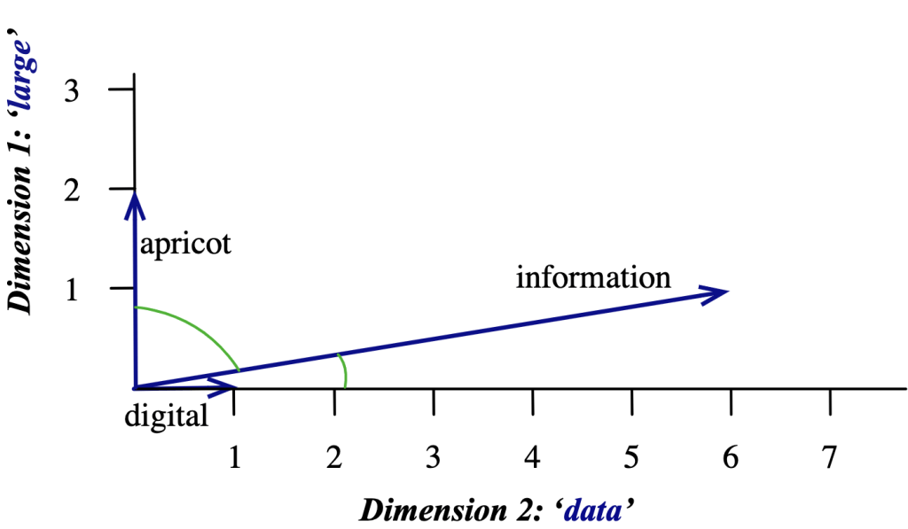
Fig. 85 Cosine similarity between two vectors

This way, using the distributional hypothesis and applying different methods to define and measure context, we can effectively determine word similarities, which is fundamental to numerous NLP tasks.

Pointwise Mutual Information (PMI)

In some situations, simple co-occurrence counts may not be as informative as we’d like. For example, a word might frequently co-occur with common words like ‘the’ or ‘a’, but this doesn’t give us a lot of insight into the semantic meaning of the word in question. This is where Pointwise Mutual Information (PMI) comes in.

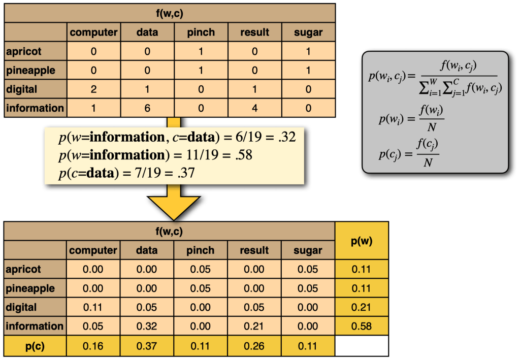
Fig. 86 PMI Formula

PMI is a measure derived from information theory that quantifies the discrepancy between the probability of two words co-occurring and the probabilities of the two words occurring independently. The PMI between a word and a context can be calculated as:

\[ PMI(w,c) = \log \frac{p(w,c)}{p(w)p(c)} \]

Where:

• \(p(w,c)\) is the probability of word \(w\) and context \(c\) co-occurring.

• \(p(w)\) and \(p(c)\) are the probabilities of word \(w\) and context \(c\) occurring independently.

To calculate these probabilities, we need the following frequencies:

• \(f(w)\): The frequency of word \(w\) in the corpus.

• \(f(c)\): The frequency of context \(c\) in the corpus.

• \(f(w,c)\): The frequency of word \(w\) co-occurring with context \(c\) in the corpus.

• \(N\): The total number of tokens in the corpus.

The probabilities can then be calculated as:

• \(p(w) = \frac{f(w)}{N}\)

• \(p(c) = \frac{f(c)}{N}\)

• \(p(w,c) = \frac{f(w,c)}{N}\)

Positive Pointwise Mutual Information (PPMI)

PMI can be negative when words co-occur less than expected by chance. However, these negative values can be unreliable, especially when working with small corpora. To address this issue, we often use Positive Pointwise Mutual Information (PPMI), which sets all negative PMI values to 0:

\[\begin{split} \text{PPMI}(w, c) = \begin{cases} \text{PMI}(w, c) & \text{ if PMI}(w, c) > 0 \\ 0 & \text{ if PMI}(w, c) \leq 0 \end{cases} \end{split}\]

PMI and Smoothing

PMI has a bias towards infrequent events. When \(P(w, c) = P(w) = P(c)\), PMI is larger for rare words with low \(P(w)\). To reduce this bias, we can apply a method called ‘Add-k smoothing’ to \(P(w, c), P(w), P(c)\), which effectively pushes all PMI values towards zero. This smoothing method affects low-probability events more, which helps reduce the bias of PMI towards infrequent events.

In summary, PMI and its variant PPMI are powerful tools for quantifying the statistical significance of word co-occurrences, and are especially useful for tasks involving semantic similarity and word association. However, they are not without their limitations, and it’s important to be aware of these when applying them in practice.