BERT: Visualizing Attention

BertViz is a powerful visualization tool designed to help users understand and interpret the inner workings of the BERT model and its variants. By providing insights into the attention mechanisms, multi-head attention, and self-attention layers, BertViz enables researchers, practitioners, and enthusiasts to better comprehend the complex relationships BERT captures within a given input text.

Installation

To install BertViz, run the following command:

pip install bertviz

%pip install bertviz

Usage

We first import the necessary libraries and modules from bertviz, transformers, and utils. We then specify the BERT model version (bert-base-uncased), and load the tokenizer and model using the AutoTokenizer and AutoModel classes from the transformers library.

%config InlineBackend.figure_format='retina'

from bertviz import model_view, head_view
from bertviz.neuron_view import show
from transformers import AutoTokenizer, AutoModel, utils

utils.logging.set_verbosity_error()  # Suppress standard warnings

model_version = "bert-base-uncased"
tokenizer = AutoTokenizer.from_pretrained(model_version)
model = AutoModel.from_pretrained(model_version, output_attentions=True)

/home/yjlee/.cache/pypoetry/virtualenvs/lecture-_dERj_9R-py3.8/lib/python3.8/site-packages/tqdm/auto.py:21: TqdmWarning: IProgress not found. Please update jupyter and ipywidgets. See https://ipywidgets.readthedocs.io/en/stable/user_install.html
  from .autonotebook import tqdm as notebook_tqdm
Downloading (…)okenizer_config.json: 100%|██████████| 28.0/28.0 [00:00<00:00, 5.17kB/s]
Downloading (…)lve/main/config.json: 100%|██████████| 570/570 [00:00<00:00, 149kB/s]
Downloading (…)solve/main/vocab.txt: 100%|██████████| 232k/232k [00:00<00:00, 5.65MB/s]
Downloading (…)/main/tokenizer.json: 100%|██████████| 466k/466k [00:00<00:00, 2.65MB/s]
Downloading pytorch_model.bin: 100%|██████████| 440M/440M [00:09<00:00, 47.8MB/s] 

Next, we define two sentences, sentence_a and sentence_b, which will serve as the input text for the visualization. We tokenize the sentences using the tokenizer.encode() function and pass them as input to the BERT model. The model processes the input and returns the attention weights as part of the output.

Now that we have the attention weights and tokenized input, we can visualize the attention mechanisms using bertviz. There are three primary visualization options available in bertviz: model_view, head_view, and neuron_view. To use any of these visualizations, you can call the corresponding function and pass in the required parameters.

sentence_a = "I went to the store."
sentence_b = "At the store, I bought fresh strawberries."

inputs = tokenizer.encode(
    [sentence_a, sentence_b],
    return_tensors="pt",
)
outputs = model(inputs)
attention = outputs[-1]
tokens = tokenizer.convert_ids_to_tokens(inputs[0])

For example, to use the head_view visualization, you can call the head_view function as follows:

head_view(attention, tokens)

head_view(attention, tokens)

Layer:

Similarly, for the model_view, you can use the following calls:

model_view(attention, tokens)

By executing any of these visualization functions, you can interactively explore the attention patterns in BERT and gain insights into how the model processes the input text.

Explaining BERT’s attention patterns

Let’s explore the attention patterns of various layers of the BERT (the BERT-Base, uncased version).

Sentence A: I went to the store.

Sentence B: At the store, I bought fresh strawberries.

BERT uses WordPiece tokenization and inserts special classifier ([CLS]) and separator ([SEP]) tokens, so the actual input sequence is:

[CLS] I went to the store . [SEP] At the store , I bought fresh straw ##berries . [SEP]

from bertviz.transformers_neuron_view import BertModel, BertTokenizer
from bertviz.neuron_view import show

model_type = "bert"
do_lower_case = True
neuron_model = BertModel.from_pretrained(model_version, output_attentions=True)
neuron_tokenizer = BertTokenizer.from_pretrained(
    model_version, do_lower_case=do_lower_case
)

show(
    neuron_model, model_type, neuron_tokenizer, sentence_a, sentence_b, layer=2, head=0
)

inputs = tokenizer.encode(
    ["I went to the store.", "At the store, I bought fresh strawberries."],
    return_tensors="pt",
)
outputs = model(inputs)
attention = outputs[-1]
tokens = tokenizer.convert_ids_to_tokens(inputs[0])

What does BERT actually learn?

Delimiter-focused attention patterns

This pattern serves as a kind of “no-op”; an attention head focuses on the [SEP] tokens when it can’t find anything else to focus on.

How exactly is BERT able to fixate on the [SEP] tokens? The answer lies in the query and key vectors.

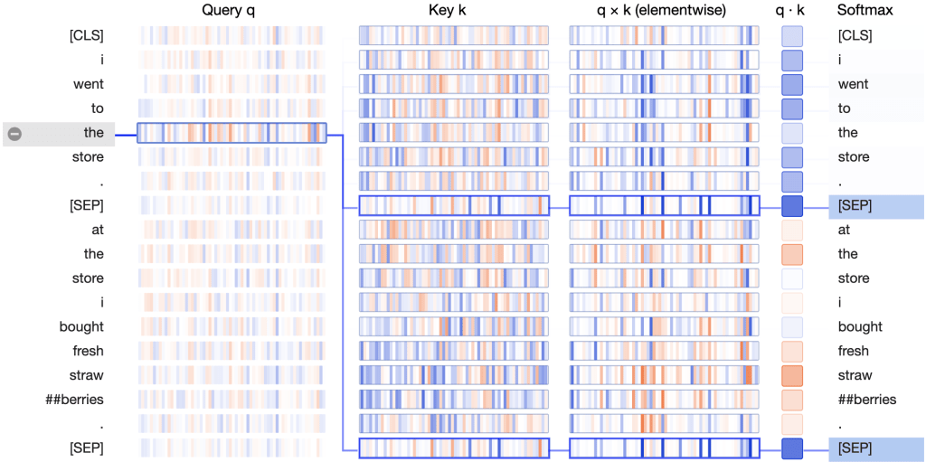
In the Key column, the key vectors for the two occurrences of [SEP] carry a distinctive signature: they both have a small number of active neurons with strongly positive (blue) or negative (orange) values, and a larger number of neurons with values close to zero (light blue/orange or white):

The query vectors tend to match the [SEP] key vectors along those active neurons, resulting in high values for the elementwise product q×k, as in this example:

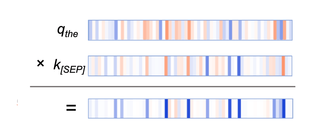
The query vectors for the other words follow a similar pattern: they match the [SEP] key vector along the same set of neurons. Thus it seems that BERT has designated a small set of neurons as “[SEP]-matching neurons,” and the query vectors assigned values that match the [SEP] key vectors at these positions.

Select layer 6, head 4. In this pattern, attention is directed to the delimiter tokens, [CLS] and [SEP].

• For example, most of the attention is directed to [SEP].

head_view(attention, tokens, layer=6, heads=[4])

Bag of Words attention pattern

In this pattern, attention is divided fairly evenly across all words in the same sentence:

BERT is essentially computing a bag-of-words embedding by taking an (almost) unweighted average of the word embeddings in the same sentence.

How does BERT finesse the queries and keys to form this attention pattern? Let’s again turn to the neuron view:

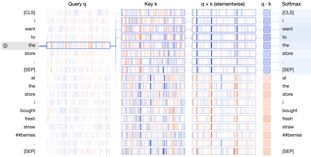
In the \(q×k\) column, we see a clear pattern: a small number of neurons (2–4) dominate the calculation of the attention scores. When query and key vector are in the same sentence (the first sentence, in this case), the product shows high values (blue) at these neurons. When query and key vector are in different sentences, the product is strongly negative (orange) at these same positions, as in this example:

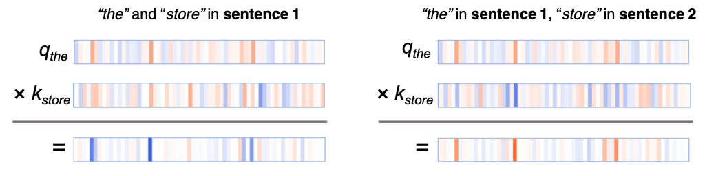
When query and key are both from sentence 1, they tend to have values with the same sign along the active neurons, resulting in a positive product. When the query is from sentence 1, and the key is from sentence 2, the same neurons tend to have values with opposite signs, resulting in a negative product.

How does BERT know the concept of “sentence”, especially in the first layer of the network before higher-level abstractions are formed? As mentioned earlier, BERT accepts special [SEP] tokens that mark sentence boundaries. Additionally, BERT incorporates sentence-level embeddings that are added to the input layer. The information encoded in these sentence embeddings flows to downstream variables, i.e. queries and keys, and enables them to acquire sentence-specific values.

Select layer 0, head 0

head_view(attention, tokens, layer=0, heads=[0])

Next-word attention pattern

It makes sense that the model would focus on the next word, because adjacent words are often the most relevant for understanding a word’s meaning in context. Traditional n-gram language models are based on this same intuition.

Let’s check out the neuron view for this pattern:

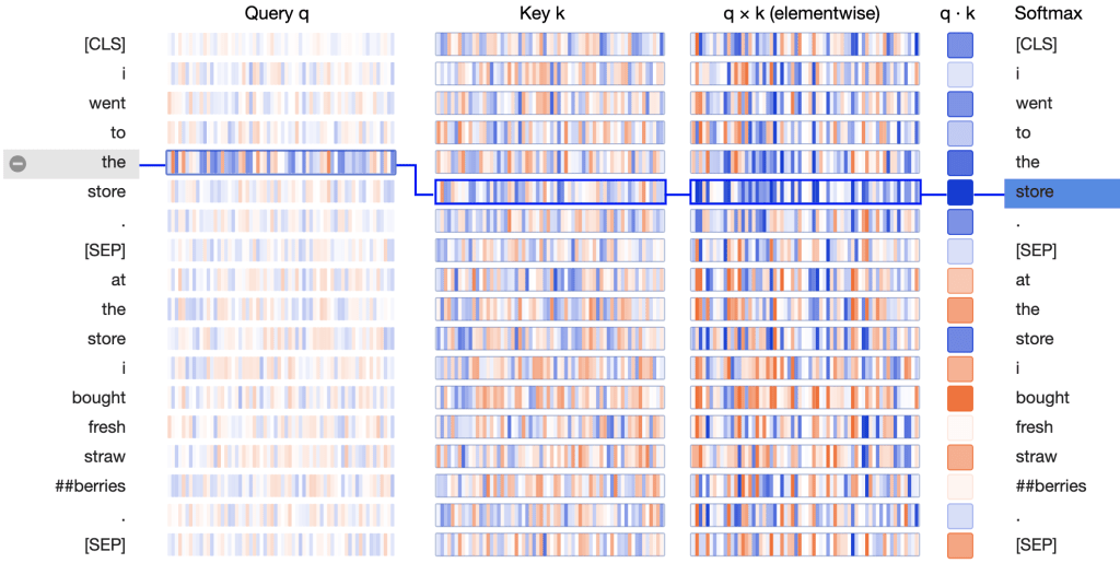
We see that the product of the query vector for “the” and the key vector for “store” (the next word) is strongly positive across most neurons. For tokens other than the next token, the key-query product contains some combination of positive and negative values. The result is a high attention score between “the” and “store”.

For this attention pattern, a large number of neurons figure into the attention score, and these neurons differ depending on the token position, as illustrated here:

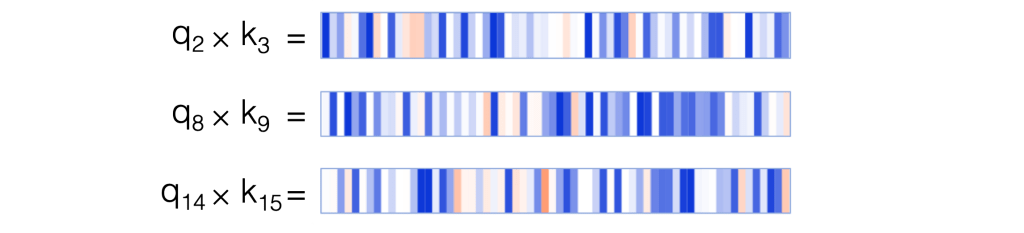
This behavior differs from the delimiter-focused and the sentence-focused attention patterns, in which a small, fixed set of neurons determine the attention scores. For those two patterns, only a few neurons are required because the patterns are so simple, and there is little variation in the words that receive attention. In contrast, the next-word attention pattern needs to track which of the 512 words receives attention from a given position, i.e., which is the next word. To do so it needs to generate queries and keys such that each query vector matches with a unique key vector from the 512 possibilities. This would be difficult to accomplish using a small subset of neurons.

How is BERT able to generate these position-aware queries and keys?

• The answer lies in BERT’s position embeddings, which are added to the word embeddings at the input layer.

• BERT learns a separate position embedding for each position in the sequence, and adds these to the word embeddings.

• This position information flows to downstream variables, i.e. queries and keys, and enables them to acquire position-specific values.

Select layer 2, head 0. (The selected head is indicated by the highlighted square in the color bar at the top.) Most of the attention at a particular position is directed to the next token in the sequence.

• If you do not select any token, the visualization shows the attention pattern for all tokens in the sequence.

• If you select a token, the visualization shows the attention pattern for the selected token.

• If you select a token i, virtually all the attention is directed to the next token went.

• The [SEP] token disrupts the next-token attention pattern, as most of the attention from [SEP] is directed to [CLS] (the first token in the sequence) rather than the next token.

• This pattern, attention to the next token, appears to work primarily within a sentence.

• This pattern is related to the idea of a recurrent neural network (RNN) that is trained to predict the next word in a sequence.

head_view(attention, tokens, layer=2, heads=[0])

Attention to previous word

Select layer 6, head 11. In this pattern, much of the attention is directed to the previous token in the sequence.

• For example, most of the attention from went is directed to the previous token i.

• The pattern is not as distinct as the next-token pattern, but it is still present.

• Some attention is also dispersed to other tokens in the sequence, especially to the [SEP] token.

• This pattern is also related to the idea of an RNN, in this case the forward direction of an RNN.

head_view(attention, tokens, layer=6, heads=[11])

Attention to identical/related words pattern

Select layer 2, head 6. In this pattern, much of the attention is directed to identical or related words, including the source word itself.

• For example, most of the attention for the first occurrence of store is directed to itself and to the second occurrence of store.

• This pattern is not as distict as some of the other patterns.

head_view(attention, tokens, layer=2, heads=[6])

Attention to identical/related words in other sentence

Select layer 10, head 10. In this pattern, much of the attention is directed to identical or related words in the other sentence.

• For example, most of the attention of store in the second sentence is directed to store in the first sentence.

• This is helpful for the next sentence prediction task, which is one of the pre-training tasks for BERT.

head_view(attention, tokens, layer=10, heads=[10])

Attention to other words predictive of word

Select layer 2, head 1. In this pattern, attention seems to be directed to other words that are predictive of the source word, excluding the source word itself.

• For example, most of the attention for straw is directed to ##berries, and most of the attention from ##berries is focused on straw.

head_view(attention, tokens, layer=2, heads=[1])

References

• Deconstructing BERT