Lab: Topic Modeling#
The problem#
In this example, we will perform topic modeling on a dataset of newsgroup documents using two matrix factorization techniques: Non-negative Matrix Factorization (NMF) and Singular Value Decomposition (SVD).
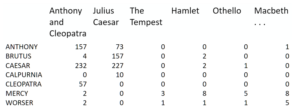
Term-document matrix:
We start by creating a term-document matrix, which represents the frequency of terms in each document. The goal is to decompose this matrix into the product of one tall, thin matrix and one wide, short matrix (possibly with a diagonal matrix in between).
It is important to note that this representation does not consider word order or sentence structure and is an example of a bag of words approach.
Motivation#
The idea behind matrix factorization is to find an optimal way of representing the original term-document matrix using lower-dimensional matrices that capture the latent topic structure in the data.
We will use a dataset of newsgroup documents belonging to several different categories and find topics (groups of words) for them. Knowing the actual categories helps us evaluate whether the discovered topics make sense.
We will try this with two different matrix factorizations: Singular Value Decomposition (SVD) and Non-negative Matrix Factorization (NMF).
Data source: The dataset used in this example is the 20 Newsgroups dataset, which contains 18,000 newsgroup posts across 20 topics. Newsgroups were popular discussion groups on Usenet in the 80s and 90s before the web took off. We will focus on four categories for this example: “alt.atheism”, “talk.religion.misc”, “comp.graphics”, and “sci.space”. To remove noise from the data, we will exclude headers, footers, and quotes from the posts.
# install the necessary packages
%pip install scikit-learn
Looking in indexes: https://pypi.org/simple, https://pypi.ngc.nvidia.com
Collecting scikit-learn
  Downloading scikit_learn-1.2.2-cp38-cp38-manylinux_2_17_x86_64.manylinux2014_x86_64.whl (9.8 MB)
     ━━━━━━━━━━━━━━━━━━━━━━━━━━━━━━━━━━━━━━━━ 9.8/9.8 MB 54.8 MB/s eta 0:00:00a 0:00:01
?25hRequirement already satisfied: joblib>=1.1.1 in /home/yjlee/.cache/pypoetry/virtualenvs/lecture-_dERj_9R-py3.8/lib/python3.8/site-packages (from scikit-learn) (1.2.0)
Requirement already satisfied: scipy>=1.3.2 in /home/yjlee/.cache/pypoetry/virtualenvs/lecture-_dERj_9R-py3.8/lib/python3.8/site-packages (from scikit-learn) (1.9.3)
Collecting threadpoolctl>=2.0.0
  Downloading threadpoolctl-3.1.0-py3-none-any.whl (14 kB)
Requirement already satisfied: numpy>=1.17.3 in /home/yjlee/.cache/pypoetry/virtualenvs/lecture-_dERj_9R-py3.8/lib/python3.8/site-packages (from scikit-learn) (1.23.5)
Installing collected packages: threadpoolctl, scikit-learn
Successfully installed scikit-learn-1.2.2 threadpoolctl-3.1.0

[notice] A new release of pip is available: 23.0 -> 23.0.1
[notice] To update, run: pip install --upgrade pip
Note: you may need to restart the kernel to use updated packages.
%config InlineBackend.figure_format='retina'
# import the necessary packages
import numpy as np
import nltk
from sklearn.datasets import fetch_20newsgroups
from sklearn import decomposition
from scipy import linalg
import matplotlib.pyplot as plt

nltk.download('stopwords')
nltk.download('wordnet')
nltk.download('omw-1.4')
[nltk_data] Downloading package stopwords to /home/yjlee/nltk_data...
[nltk_data]   Package stopwords is already up-to-date!
[nltk_data] Downloading package wordnet to /home/yjlee/nltk_data...
[nltk_data]   Package wordnet is already up-to-date!
[nltk_data] Downloading package omw-1.4 to /home/yjlee/nltk_data...
[nltk_data]   Package omw-1.4 is already up-to-date!
True
categories = ["alt.atheism", "talk.religion.misc", "comp.graphics", "sci.space"]
remove = ("headers", "footers", "quotes")
newsgroups_train = fetch_20newsgroups(
    subset="train", categories=categories, remove=remove
)
newsgroups_test = fetch_20newsgroups(
    subset="test", categories=categories, remove=remove
)
newsgroups_train.filenames.shape, newsgroups_train.target.shape
((2034,), (2034,))
Let’s take a look at some of the data. Can you guess which category these messages belong to?
print("\n".join(newsgroups_train.data[:2]))
Hi,

I've noticed that if you only save a model (with all your mapping planes
positioned carefully) to a .3DS file that when you reload it after restarting
3DS, they are given a default position and orientation.  But if you save
to a .PRJ file their positions/orientation are preserved.  Does anyone
know why this information is not stored in the .3DS file?  Nothing is
explicitly said in the manual about saving texture rules in the .PRJ file.
I'd like to be able to read the texture rule information, does anyone have
the format for the .PRJ file?

Is the .CEL file format available from somewhere?

Rych


Seems to be, barring evidence to the contrary, that Koresh was simply
another deranged fanatic who thought it neccessary to take a whole bunch of
folks with him, children and all, to satisfy his delusional mania. Jim
Jones, circa 1993.


Nope - fruitcakes like Koresh have been demonstrating such evil corruption
for centuries.
The target attribute is the integer index of the category.
np.array(newsgroups_train.target_names)[newsgroups_train.target[:3]]
array(['comp.graphics', 'talk.religion.misc', 'sci.space'], dtype='<U18')
In this example, we will use NMF and SVD to decompose the term-document matrix and extract latent topics from the newsgroup documents. By comparing the discovered topics with the actual categories, we can evaluate the effectiveness of these matrix factorization techniques in uncovering meaningful topic structures in text data.
newsgroups_train.target[:10]
array([1, 3, 2, 0, 2, 0, 2, 1, 2, 1])
num_topics, num_top_words = 6, 8
Note
Stopwords
Stopwords are extremely common words that appear to have little value in helping to identify or match documents based on user needs. In text processing and information retrieval, these words are often excluded from the analysis to reduce noise and improve efficiency. Examples of stopwords include “a”, “an”, “the”, “and”, and “in”.
Over time, the trend in information retrieval systems has shifted from using large stop lists (200-300 terms) to very small stop lists (7-12 terms), and eventually to not using stop lists at all. Web search engines typically do not use stop lists.
Stemming and Lemmatization
Stemming and lemmatization are text preprocessing techniques that aim to generate the root form of words. This is particularly useful in information retrieval, as it helps group similar words together and improves search accuracy. Consider the following words:
organize, organizes, and organizing
democracy, democratic, and democratization
Both stemming and lemmatization aim to reduce these words to their base forms, making it easier to identify their similarities.
Lemmatization uses linguistic rules and knowledge about a language to generate the root form of words. The resulting tokens are actual words that carry meaning in the language. In contrast, stemming is a simpler and more heuristic-based approach that truncates words by chopping off their ends. The resulting tokens may not always be real words. As a result, stemming is faster than lemmatization but may not be as accurate.
In summary, stopwords, stemming, and lemmatization are essential techniques in text processing and information retrieval. They help reduce noise, improve efficiency, and enhance the overall effectiveness of search and topic modeling tasks by simplifying the input text and generating meaningful word representations.
from nltk.corpus import stopwords

STOPWORDS = stopwords.words("english")
print(len(STOPWORDS))
print(STOPWORDS[:10])
179
['i', 'me', 'my', 'myself', 'we', 'our', 'ours', 'ourselves', 'you', "you're"]
from nltk import stem

wnl = stem.WordNetLemmatizer()
porter = stem.porter.PorterStemmer()

word_list = ["feet", "foot", "foots", "footing"]
[wnl.lemmatize(word) for word in word_list]
['foot', 'foot', 'foot', 'footing']
[porter.stem(word) for word in word_list]
['feet', 'foot', 'foot', 'foot']
Data Processing#
In this step, we will process the newsgroup data by extracting word counts using scikit-learn’s CountVectorizer. This method will create a term-document matrix representing the frequency of terms in each document. In a later lesson, we will learn how to create our own version of CountVectorizer to gain a better understanding of what happens under the hood.
from sklearn.feature_extraction.text import CountVectorizer

# Initialize the CountVectorizer with English stopwords
vectorizer = CountVectorizer(stop_words="english")

# Fit the vectorizer to the newsgroups_train.data and transform the text data
vectors = vectorizer.fit_transform(
    newsgroups_train.data
).todense()  # (documents, vocab)

# Print the shape of the term-document matrix (documents, vocabulary)
print(len(newsgroups_train.data), vectors.shape)

# Retrieve the vocabulary from the vectorizer
vocab = np.array(vectorizer.get_feature_names_out())

# Print the shape of the vocabulary
print(vocab.shape)

# Display the last 10 terms in the vocabulary
print(vocab[-10:])
2034 (2034, 26576)
(26576,)
['zurich' 'zurvanism' 'zus' 'zvi' 'zwaartepunten' 'zwak' 'zwakke' 'zware'
 'zwarte' 'zyxel']
In this code snippet, we first import CountVectorizer from scikit-learn’s feature_extraction.text module. We then initialize the CountVectorizer object, specifying that we want to remove English stopwords from the text data. Next, we fit the vectorizer to the training data and transform the text data into a term-document matrix. Finally, we retrieve the vocabulary from the vectorizer and display its shape and the last 10 terms.
By applying CountVectorizer to the newsgroup data, we can transform the text data into a structured format suitable for further analysis using NMF and SVD.
Singular Value Decomposition (SVD)#
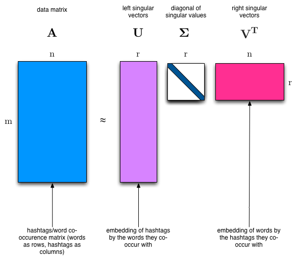
SVD is a matrix factorization technique that can be used to identify latent topics in a term-document matrix. We expect the topics to be orthogonal since words that appear frequently in one topic should appear less frequently in others, making them suitable for separating topics.
The SVD algorithm factorizes a matrix into one matrix with orthogonal columns and one with orthogonal rows, along with a diagonal matrix that contains the relative importance of each factor. SVD is an exact decomposition as the resulting matrices fully cover the original matrix. It is widely used in data science for tasks such as semantic analysis, collaborative filtering, data compression, and principal component analysis. Latent Semantic Analysis (LSA) also employs SVD.
Latent Semantic Analysis (LSA) uses SVD.
%%time
from scipy import linalg

# Perform SVD on the term-document matrix
U, s, Vh = linalg.svd(vectors, full_matrices=False)

# Print the shapes of the resulting matrices
print(U.shape, s.shape, Vh.shape)
(2034, 2034) (2034,) (2034, 26576)
CPU times: user 9min 13s, sys: 7min 22s, total: 16min 35s
Wall time: 17.8 s
In this code snippet, we import the linalg module from SciPy and use its svd function to perform SVD on the term-document matrix. We then print the shapes of the resulting matrices U, s, and Vh.
num_top_words = 8


def show_topics(a):
    # Helper function to retrieve top words for each topic
    top_words = lambda t: [vocab[i] for i in np.argsort(t)[: -num_top_words - 1 : -1]]
    topic_words = [top_words(t) for t in a]
    return [" ".join(t) for t in topic_words]
# Display the top topics extracted using SVD
show_topics(Vh[:10])
['critus ditto propagandist surname galacticentric kindergarten surreal imaginative',
 'jpeg gif file color quality image jfif format',
 'graphics edu pub mail 128 3d ray ftp',
 'jesus god matthew people atheists atheism does graphics',
 'image data processing analysis software available tools display',
 'god atheists atheism religious believe religion argument true',
 'space nasa lunar mars probe moon missions probes',
 'image probe surface lunar mars probes moon orbit',
 'argument fallacy conclusion example true ad argumentum premises',
 'space larson image theory universe physical nasa material']
In this part, we define a function show_topics to display the top words associated with each topic. We then use this function to display the top topics extracted using SVD. The results match the expected clusters, even though this is an unsupervised algorithm - meaning we never provided information about the grouping of our documents during the process.
Non-negative Matrix Factorization (NMF)#
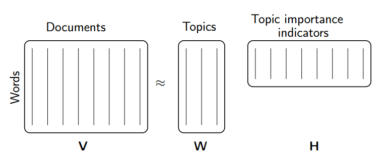
In contrast to constraining our factors to be orthogonal as in SVD, we can constrain them to be non-negative. NMF is a factorization of a non-negative data set \(V\) into non-negative matrices \(W\) and \(H\): \(V=WH\). Often, positive factors are more easily interpretable, contributing to NMF’s popularity.
NMF is a non-exact factorization that factors a matrix into one skinny positive matrix and one short positive matrix. It is NP-hard and non-unique, with various versions created by adding different constraints.
NMF Applications#
NMF has been applied in various fields, such as:
NMF using scikit-learn#
%%time
from sklearn import decomposition

# Perform NMF on the term-document matrix
m, n = vectors.shape
d = 5  # num topics

clf = decomposition.NMF(n_components=d, random_state=1)

W1 = clf.fit_transform(np.asarray(vectors))
H1 = clf.components_
CPU times: user 1min 36s, sys: 1min 33s, total: 3min 9s
Wall time: 2.86 s
# Display the top topics extracted using NMF
show_topics(H1)
['jpeg image gif file color images format quality',
 'edu graphics pub mail 128 ray ftp send',
 'space launch satellite nasa commercial satellites year market',
 'jesus god people matthew atheists does atheism said',
 'image data available software processing ftp edu analysis']
In this code snippet, we import the decomposition module from scikit-learn and use its NMF class to perform NMF on the term-document matrix. We then display the top topics extracted using NMF.
Note
For NMF, the matrix needs to be at least as tall as it is wide, or we get an error with
fit_transform.You can use
min_dfinCountVectorizerto only consider words that appear in at least k of the split texts.
Truncated SVD#
When we calculated NMF, we saved a lot of time by only calculating the subset of columns we were interested in. We can achieve a similar benefit with SVD by using truncated SVD. Truncated SVD focuses on the vectors corresponding to the largest singular values, which can save computation time.
Shortcomings of classical algorithms for decomposition:#
Matrices can be “stupendously big.”
Data are often missing or inaccurate. Spending extra computational resources may not be worthwhile when the imprecision of input limits the precision of the output.
Data transfer plays a significant role in the time complexity of algorithms. Techniques that require fewer passes over the data might be faster, even if they require more floating point operations (flops).
It is essential to take advantage of GPUs.
Advantages of randomized algorithms:#
Inherently stable.
Performance guarantees do not depend on subtle spectral properties.
The required matrix-vector products can be performed in parallel.
(source: Halko)
Timing comparison#
In the following code snippets, we compare the computation time for full SVD and randomized SVD:
%%time
# Full SVD
u, s, v = np.linalg.svd(vectors, full_matrices=False)
CPU times: user 10min 29s, sys: 10min 50s, total: 21min 20s
Wall time: 20.7 s
%%time
# Randomized SVD
u, s, v = decomposition.randomized_svd(vectors, n_components=10, random_state=123)
CPU times: user 1min 1s, sys: 2min 30s, total: 3min 32s
Wall time: 5.91 s
These code snippets demonstrate the time difference between full SVD and randomized SVD, showing that the latter can be more efficient in certain cases.