Word2Vec#
Word2Vec is a neural network architecture that was proposed by [Mikolov et al., 2013] in 2013. It is a shallow, two-layer neural network that is trained to reconstruct linguistic contexts of words.
The problem of the previous neural network is that it is computationally expensive to train. The hidden layer computes probability distribution for all the words in the vocabulary. This is because the output layer is a fully connected layer.
Word2Vec solves this problem by using a single output neuron. This is achieved by using a hierarchical softmax or negative sampling method.
Main idea#
Use a
binary classifierto predict which words appear in the context of (i.e. near) a target word.The
parameters of that classifierprovide a dense vector representation of the target word (embedding).Words that appear in similar contexts (that have high distributional similarity) will have very similar vector representations.
These models can be trained on large amounts of raw text (and pre-trained embeddings can be downloaded).
Negative sampling#
Train a binary classifier that decides whether a target word t appears in the context of other words \(c_{1..k}\)
Context: the set of k words near (surrounding) tTreat the target word t and any word that actually appears in its context in a real corpus as
positiveexamplesTreat the target word t and randomly sampled words that don’t appear in its context as
negativeexamplesTrain a
binary logistic regressionclassifier to distinguish these casesThe
weightsof this classifier depend on thesimilarityof t and the words in \(c_{1..k}\)
Two models#
Continuous Bag of Words (CBOW): predicts the target word from the context words.
Skip-gram: predicts the context words from the target word.
When to use the skip-gram model and when to use CBOW?#
CBOW is faster to train than skip-gram.
Skip-gram is better at capturing rare words and their contexts.
CBOW is better at capturing common words and their contexts.
Skip-gram works better with small datasets.
Therefore, the choice of model depends on the kind of problem you are trying to solve.
Skip-gram model#
The skip-gram model is the same as the CBOW model with one difference: it predicts the context words from the target word.
In the above figure, \(w[t]\) is the target word, and \(w[t-2], w[t-1], w[t+1], w[t+2]\) are the context words, where \(t\) is the location of the target word in the sentence.
The model predicts the probability of a word being a context word given the target word. The output probabilities explain how likely a word is to be close to the target word.
This shallow neural network architecture is called a skip-gram model because it predicts the context words from the target word.
We don’t use this trained network for prediction. Instead, we use the weights of the embedding layer as the word embeddings.
Step 0: Prepare the data#
%config InlineBackend.figure_format='retina'

from ekorpkit import eKonf

cfg = eKonf.compose('path')
cfg.cache.uri = 'https://github.com/entelecheia/ekorpkit-book/raw/main/assets/data/us_equities_news_sampled.zip'
corpus = eKonf.load_data("us_equities_news_sampled.parquet", cfg.cached_path)
sentences = corpus.text[2].lower().split("\n")
words = " ".join(sentences).split()
sentences
['chip name micron technology inc nasdaq mu is higher on two new price target hikes from analysts specifically bmo lifted its price target to 60 from 50 while cowen boosted its estimate to 46 from 38 these two bull notes come just one day before mu s fiscal fourth quarter earnings report due out after the close tomorrow sept 26',
 'this puts the consensus micron nasdaq mu 12 month target price at 51 59 which sits just atop the stock s sept 11 of 51 39 and represents a 7 premium to mu s current perch at 49 22 up 1 5 on the day meanwhile 14 brokerages in coverage call the equity a buy or better and 10 say it s a hold or worse',
 'it s no surprise that most analysts are optimistic ahead of mu s quarterly reveal the semiconductor name tends to do quite well the day after earnings in fact only three of its last eight post earnings moves were negative and the equity managed a 13 3 next day pop on in june this time around the options market is pricing in an 11 4 swing for friday s trading regardless of direction much wider than the 6 9 move the equity has averaged over the past two years',
 'while mu tends to pop the day after earnings investors might want to look out a little further data from schaeffer s senior quantitative analyst rocky white shows the equity is one of the after the fed cuts rates twice in 60 days which just occurred last week looking at data from 1984 mu finished the higher one month later after only 33 of previous signals averaging an underwhelming one month gain of 1 04',
 'drilling down the options pits have seen an uptick in bearish activity today with 47 000 puts across the tape two times the intraday average compared to 25 000 calls a massive portion of these contracts have changed hands at the october 43 put where positions are possibly being bought to open this means traders are expecting a big swing lower through expiration at the close on friday oct 18']
Step 1: Setting target and context variable#
Since skipgram takes a single context word and n number of target variables, we just need to flip the CBOW from the previous model.
when the window size is 1, we take one word before and after the target word.
For example, if we have the sentence “I like deep learning because it is fun”, and the window size is 1, the function will return the following list:
[['like', 'I'],
 ['like', 'deep'],
 ['deep', 'like'],
 ['deep', 'learning'],
 ['learning', 'deep'],
 ['learning', 'because'],
 ...
]
def skipgram(words, window_size=1):
    skip_grams = []
    for i in range(window_size, len(words) - window_size):
        target = words[i]
        context = [words[i - window_size], words[i + window_size]]
        for w in context:
            skip_grams.append([target, w])

    return skip_grams
skipgram("I like deep learning because it is fun".split(), 1)
[['like', 'I'],
 ['like', 'deep'],
 ['deep', 'like'],
 ['deep', 'learning'],
 ['learning', 'deep'],
 ['learning', 'because'],
 ['because', 'learning'],
 ['because', 'it'],
 ['it', 'because'],
 ['it', 'is'],
 ['is', 'it'],
 ['is', 'fun']]
Step 2: Building the model#
import torch
import torch.nn as nn


class skipgramModel(nn.Module):
    def __init__(self, vocab_size, embedding_size, word_to_ix):
        super(skipgramModel, self).__init__()
        self.embedding = nn.Embedding(vocab_size, embedding_size)
        self.W = nn.Linear(embedding_size, embedding_size, bias=False)
        self.WT = nn.Linear(embedding_size, vocab_size, bias=False)
        self.word_to_ix = word_to_ix

    def forward(self, X):
        embeddings = self.embedding(X)
        hidden_layer = nn.functional.relu(self.W(embeddings))
        output_layer = self.WT(hidden_layer)
        return output_layer

    def get_word_emdedding(self, word):
        word = torch.tensor([self.word_to_ix[word]])
        return self.embedding(word).view(1, -1)
Step 3: Loss and optimization function#
import torch.optim as optim

word_list = list(set(words))
word_to_id = {w: i for i, w in enumerate(word_list)}
id_to_word = {i: w for w, i in word_to_id.items()}
vocab_size = len(word_list)
print("vocab_size:", vocab_size)

batch_size = 2  # mini-batch size
embedding_size = 5  # embedding size

model = skipgramModel(vocab_size, embedding_size, word_to_id)

criterion = nn.CrossEntropyLoss()
optimizer = optim.Adam(model.parameters(), lr=0.01)
vocab_size: 222
Step 4: Training the model#
import numpy as np
from tqdm.auto import tqdm


def words_to_vector(words, word_to_ix):
    idxs = [word_to_ix[w] for w in words]
    return torch.tensor(idxs, dtype=torch.long)


def random_batch(skip_grams, batch_size=2):
    random_inputs = []
    random_labels = []
    random_index = np.random.choice(range(len(skip_grams)), batch_size, replace=False)

    for i in random_index:
        random_inputs.append(skip_grams[i][0])  # target
        random_labels.append(skip_grams[i][1])  # context word

    return random_inputs, random_labels


for epoch in tqdm(range(150000), total=len(skipgram(words))):
    input_batch, target_batch = random_batch(skipgram(words), batch_size)
    input_batch = torch.LongTensor(words_to_vector(input_batch, word_to_id))
    target_batch = torch.LongTensor(words_to_vector(target_batch, word_to_id))

    optimizer.zero_grad()
    output = model(input_batch)

    # output : [batch_size, voc_size], target_batch : [batch_size] (LongTensor, not one-hot)
    loss = criterion(output, target_batch)
    if (epoch + 1) % 10000 == 0:
        print("Epoch:", "%04d" % (epoch + 1), "cost =", "{:.6f}".format(loss))

    loss.backward(retain_graph=True)
    optimizer.step()
Epoch: 10000 cost = 3.896727
Epoch: 20000 cost = 2.242064
Epoch: 30000 cost = 3.617461
Epoch: 40000 cost = 4.317378
Epoch: 50000 cost = 2.380702
Epoch: 60000 cost = 4.073981
Epoch: 70000 cost = 3.560866
Epoch: 80000 cost = 4.322421
Epoch: 90000 cost = 2.438971
Epoch: 100000 cost = 4.790970
Epoch: 110000 cost = 4.703344
Epoch: 120000 cost = 2.545708
Epoch: 130000 cost = 2.590156
Epoch: 140000 cost = 2.531536
Epoch: 150000 cost = 2.791655
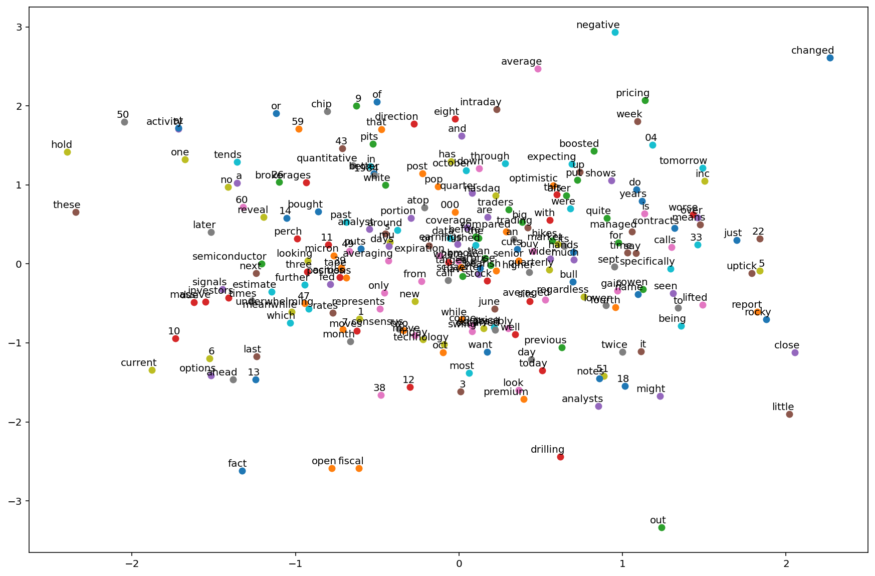
Visualizing the embeddings#
import matplotlib.pyplot as plt


plt.figure(figsize=(15, 10))

for w in word_list:
    x = model.get_word_emdedding(w).detach().data.numpy()[0][0]
    y = model.get_word_emdedding(w).detach().data.numpy()[0][1]
    plt.scatter(x, y)
    plt.annotate(
        w, xy=(x, y), xytext=(5, 2), textcoords="offset points", ha="right", va="bottom"
    )
plt.show()
Evaluation#
def skipgram_test(test_data, model):
    correct_ct = 0

    for i in range(len(test_data)):
        input_batch, target_batch = random_batch(test_data, batch_size)
        input_batch = torch.LongTensor(words_to_vector(input_batch, word_to_id))
        target_batch = torch.LongTensor(words_to_vector(target_batch, word_to_id))

        model.zero_grad()
        _, predicted = torch.max(model(input_batch), 1)

        if predicted[0] == target_batch[0]:
            correct_ct += 1

    print(
        "Accuracy: {:.1f}% ({:d}/{:d})".format(
            correct_ct / len(test_data) * 100, correct_ct, len(test_data)
        )
    )
skipgram_test(skipgram(words), model)
Accuracy: 13.0% (93/716)
pred = ["earnings"]

model_pred = []
e = 0
model_pred.append(pred[0])

while e < 6:
    word = id_to_word[
        torch.argmax(model(torch.LongTensor([word_to_id[model_pred[-1]]]))).item()
    ]
    model_pred.append(word)
    e += 1

" ".join(model_pred)
'earnings quarter fourth october 9 and senior'
The skip-gram model increases computational complexity because it has to predict nearby words based on the number of neighboring words. The more distant words tend to be slightly less related to the current word.
Continuous Bag of Words (CBOW)#
The CBOW model predicts the target word from the context words.
This model reduces the complexity of calculating the probability distribution for all the words in the vocabulary to the \(\log_2(V)\) complexity of calculating the probability distribution for the target word.
Architecture#
The input layer is the context words.
The input is \(C\) context words, each represented as a one-hot vector of size \(V\), where \(V\) is the size of the vocabulary, yielding a \(C \times V\) matrix.
Each row of the matrix is multiplied by the weight matrix \(W\) of size \(V \times N\), where \(N\) is the size of the embedding.
The resulting matrix is summed up to get a vector of size \(N\).
This vector is passed through a softmax layer to get the probability distribution of the target word.
The learned weights of the softmax layer are the word embeddings.
Step 1: Define a function to create a context and a target word#
Define a function to create a context window with n words from the right and left of the target word.
The function should take two arguments: data and window size. The window size will define how many words we are supposed to take from the right and from the left.
The for loop: for i in range(window_size, len(words) – window_size): iterates through a range starting from the window size, i.e. 2 means it will ignore words in index 0 and 1 from the sentence, and end 2 words before the sentence ends.
Inside the for loop, we try separate context and target words and store them in a list.
For example, if we have the sentence “I like deep learning because it is fun”, and the window size is 2, the function will return the following list:
[(['I', 'like', 'learning', 'because'], 'deep'),
 (['like', 'deep', 'because', 'it'], 'learning'),
 (['deep', 'learning', 'it', 'is'], 'because'),
 (['learning', 'because', 'is', 'fun'], 'it')]
def CBOW(words, window_size=2):
    data = []
    for i in range(window_size, len(words) - window_size):
        context = [
            words[i - window_size],
            words[i - (window_size - 1)],
            words[i + (window_size - 1)],
            words[i + window_size],
        ]
        target = words[i]
        data.append((context, target))

    return data
Let’s call the function and see the output.
CBOW("I like deep learning because it is fun".split())
[(['I', 'like', 'learning', 'because'], 'deep'),
 (['like', 'deep', 'because', 'it'], 'learning'),
 (['deep', 'learning', 'it', 'is'], 'because'),
 (['learning', 'because', 'is', 'fun'], 'it')]
Step 2: Build the model#
In the CBOW model, we reduce the hidden layer to only one. So all together we have: an embedding layer, a hidden layer which passes through the ReLU layer, and an output layer.
The context words index is fed into the embedding layers, which is then passed through the hidden layer followed by the nonlinear activation layer, i.e. ReLU, and finally we get the output.
import torch
import torch.nn as nn


class CBOW_Model(torch.nn.Module):
    def __init__(self, vocab_size, embedding_dim, word_to_ix):
        super(CBOW_Model, self).__init__()
        self.word_to_ix = word_to_ix

        # out: 1 x emdedding_dim
        self.embeddings = nn.Embedding(vocab_size, embedding_dim)
        self.linear1 = nn.Linear(embedding_dim, 128)
        self.activation_function1 = nn.ReLU()

        # out: 1 x vocab_size
        self.linear2 = nn.Linear(128, vocab_size)

    def forward(self, inputs):
        embeds = sum(self.embeddings(inputs)).view(1, -1)
        out = self.linear1(embeds)
        out = self.activation_function1(out)
        out = self.linear2(out)
        return out

    def get_word_emdedding(self, word):
        word = torch.tensor([self.word_to_ix[word]])
        return self.embeddings(word).view(1, -1)
Step 3: Loss and optimization function.#
We are using the cross-entropy loss function and the SGD optimizer. You can also use the Adam optimizer.
CONTEXT_SIZE = 2  # 2 words to the left, 2 to the right
EMDEDDING_DIM = 100

# By deriving a set from `words`, we deduplicate the array
vocab = set(words)
vocab_size = len(vocab)
print("vocab_size:", vocab_size)

word_list = list(vocab)

word_to_id = {word: ix for ix, word in enumerate(vocab)}
id_to_word = {ix: word for ix, word in enumerate(vocab)}

data = CBOW(words)
model = CBOW_Model(vocab_size, EMDEDDING_DIM, word_to_id)

loss_function = nn.CrossEntropyLoss()
optimizer = torch.optim.SGD(model.parameters(), lr=0.01)
vocab_size: 222
Step 4: Training the model.#
Finally, we train the model.
words_to_vector turns words into numbers.
for epoch in range(50):
    total_loss = 0

    for context, target in data:
        context_vector = words_to_vector(context, word_to_id)

        log_probs = model(context_vector)

        total_loss += loss_function(log_probs, torch.tensor([word_to_id[target]]))

    # optimize at the end of each epoch
    optimizer.zero_grad()
    total_loss.backward()
    optimizer.step()
    if (epoch + 1) % 10 == 0:
        print(f"Epoch: {epoch}, Loss: {total_loss.item()}")
Epoch: 9, Loss: 7.895180702209473
Epoch: 19, Loss: 6.261657238006592
Epoch: 29, Loss: 5.2918782234191895
Epoch: 39, Loss: 4.626347541809082
Epoch: 49, Loss: 4.151697635650635
Visualizing the embeddings#
import matplotlib.pyplot as plt

plt.figure(figsize=(15, 10))

for w in word_list:
    x = model.get_word_emdedding(w).detach().data.numpy()[0][0]
    y = model.get_word_emdedding(w).detach().data.numpy()[0][1]
    plt.scatter(x, y)
    plt.annotate(
        w, xy=(x, y), xytext=(5, 2), textcoords="offset points", ha="right", va="bottom"
    )
plt.show()
Evaluation#
def CBOW_test(test_data, model):
    correct_ct = 0

    for context, target in data:
        context_vector = words_to_vector(context, word_to_id)
        model.zero_grad()
        predicted = torch.argmax(model(context_vector), 1)

        if predicted[0] == torch.tensor([word_to_id[target]]):
            correct_ct += 1

    print(
        "Accuracy: {:.1f}% ({:d}/{:d})".format(
            correct_ct / len(test_data) * 100, correct_ct, len(test_data)
        )
    )
CBOW_test(data, model)
Accuracy: 99.7% (355/356)
context = ["chip", "name", "technology", "inc"]
context_vector = words_to_vector(context, word_to_id)
a = model(context_vector)
print(f"Context: {context}\n")
print(f"Prediction: {id_to_word[torch.argmax(a[0]).item()]}")
Context: ['chip', 'name', 'technology', 'inc']

Prediction: micron
Improving predictive functions#
Softmax#
The equation for the softmax function is:
where \(x_i\) is the score of the target word \(w_i\) and \(c\) is the context words.
The complexity of the softmax function is \(\mathcal{O}(n)\), where \(n\) is the number of words in the vocabulary.
With a large vocabulary, say 100,000 words, the softmax function becomes very expensive to compute. For each word (\(w_i\)), we have to compute the exponential of the score of each word in the vocabulary (\(x_j\)) and then sum them up. This is \(\mathcal{O}(n)\).
Hierarchical softmax#
Hierarchical softmax is a method to reduce the complexity of the softmax function. It is a tree-based data structure that is used to represent the vocabulary.
Hierarchical softmax was introduced by Morin and Bengio in 2005, as an alternative to the full softmax function, where it replaces it with a hierarchical layer. It borrows the technique from the binary huffman tree, which reduces the complexity of calculating the probability from \(\mathcal{O}(n)\) to \(\mathcal{O}(\log_2(n))\).
The hierarchical softmax is a binary tree, where each node represents a word in the vocabulary. The root node represents the entire vocabulary. The left child represents the words that are less frequent than the parent node, and the right child represents the words that are more frequent than the parent node.
The probability of a word \(w_i\) is the product of the probabilities of the nodes on the path from the root to the leaf node that represents \(w_i\).
In the huffman tree, we no longer calculate the output embeddings \(w^\prime\). Instead, we calculate the probability of turning right or left at each node.
Noise-contrastive estimation#
Noise-contrastive estimation (NCE) is an approximation method to reduce the complexity of the softmax function. It is a sampling-based method that is used to approximate the softmax function.
NCE takes an unnormalised multinomial function (i.e. the function that has multiple labels and its output has not been passed through a softmax layer), and converts it to a binary logistic regression.
In order to learn the distribution to predict the target word (\(w_t\)) from some specific context (\(c\)), we need to create two classes: positive samples and negative samples.
The positive class contains samples from training data distribution, while the negative class contains samples from a noise distribution \(Q\), and we label them 1 and 0 respectively. Noise distribution is a unigram distribution of the training set.
For every target word given context, we generate sample noise from the distribution \(Q\) as \(Q(w)\), such that it’s \(k\) times more frequent than the samples from the training data distribution \(P(w|c)\).
The loss function is the sum of the log probabilities of the positive samples and the negative samples, and is given by:
where \(w_i\) is the \(i\)th negative sample.
As we increase the number of noise samples \(k\), the NCE derivative approaches the likelihood gradient, or the softmax function of the normalised model.
In conclusion, NCE is a way of learning a data distribution by comparing it against a noise distribution, and modifying the learning parameters such that the model \(P_{\theta}\) is closer to the noise \(P_{\text{data}}\).
Negative sampling#
Negative sampling is a sampling-based method that is used to approximate the softmax function. It simplifies the NCE method by removing the need to calculate the noise distribution \(Q\).
Negative sampling gets rid of the noise distribution \(Q\) and uses a single noise sample \(w_j\) for each target word \(w_t\).
The loss function is the sum of the log probabilities of the positive samples and the negative samples, and is given by:
where \(\sigma\) is the sigmoid function.